Notes for Machine Learning - Week 2
Contents
Linear Regression with Multiple Variables
Multivariate Linear Regression
- Multiple features (variables)
- $n$ = number of features
- $x^{(i)}$ = input (features) of $i^{th}$ training example.
- $x^{(i)}_j$ = value of feature $j$ in $i^{th}$ training example.
- Hypotesis
- Previously: $h_\theta (x) = \theta_0 + \theta_1 x$
- $h_\theta (x) = \theta_0 + \theta_1 x_1 + \theta_2 x_2 + \cdots + \theta_n x_n$
- For convenience of notation, define $x_0=1$
- $x=\begin{bmatrix}x_0 \\ x_1 \\ x_2 \\ \vdots \\ x_n \end{bmatrix}, \theta = \begin{bmatrix}\theta_0 \\ \theta_1 \\ \theta_2 \\ \vdots \\ \theta_n \end{bmatrix}, h_\theta (x) = \theta^T x$
Gradient Descent for Multiple Variables
Hypothesis: $h_\theta(x)=\theta^Tx=\theta_0 x_0 + \theta_1 x_1 + \theta_2 x_2 + \cdots + \theta_n x_n$
Parameters: $\theta_0, \theta_1, \dots ,\theta_n$
Cost function: $J(\theta_0, \theta1, \dots, \theta_n) = \frac{1}{2m} \sum^m_{i=1}\left(h\theta (x^{(i)})-y^{(i)}\right)^2$
- or $J(\theta) = \frac{1}{2m}\sum_{i=1}^{m}(\theta^T x^{(i)} - y^{(i)})^2$
Gradient descent
repeat {
$\theta_j := \theta_j - \alpha \frac{\partial}{\partial \theta_j} J(\theta_0, \dots ,\theta_n)$
(simultaneously update for every $j=0,\dots,n$)
}
or
repeat {
$\thetaj := \theta_j - \alpha \frac{1}{m} \sum^m_{i=1}\left(h\theta(x^{(i)})-y^{(i)}\right) x^{(i)}_j$
(simultaneously update for every $j=0,\dots,n$)
}
Gradient Descent in Practice
Feature Normalization
Idea: Make sure featueres are on a similar scale.
- We can speed up gradient descent by having each of our input values in roughly the same range. This is because $\theta$ will descend quickly on small ranges and slowly on large ranges, and so will oscillate inefficiently down to the optimum when the variables are very uneven.
- The way to prevent this is to modify the ranges of our input variables so that they are all roughly the same.
Example
- $x_1$ = size (0-2000 $feet^2$)
- $x_2$ = number of bedrooms (1-5)
$x_1$ has a much larger range of values than $x_2$. So the $J(\theta_1, \theta_2)$ can be a very very skewed elliptical shape. And if you run gradient descents on this cost function, your gradients may end up taking a long time and can oscillate back and forth and take a long time before it can finally find its way to the global minimum.
Feature scaling
Get every feature into approcimately $-1\le x_i \le 1$ range.
- Feature scaling involves dividing the input values by the range (i.e. the maximum value minus the minimum value) of the input variable, resulting in a new range of just 1.
These aren’t exact requirements; we are only trying to speed things up.
$-3\le x_i \le 3$ or $ -\frac{1}{3} \le x_i \le \frac{1}{3}$ just is fine.
Mean normalization
Replace $x_i$ with $x_i - \mu _i$ to make features have approximately zero mean (Do not apply to $x_0 = 1$)
- E.g. $x_1 = \frac{size -1000}{2000}, x_2 = \frac{bedrooms - 2}{5}$
- $x_i = \frac{x_i - \mu _i}{s_i}$
- $\mu _i$ is the average value of $x_i$ in training set.
- $s_i$ is the range ($x_{imax}-x_{imin}$) or standard deviation ($\sigma$)
Learning Rate
- “Debugging”: How to make sure gradient descent is working correctly
- Make a plot with *number of iterations* on the x-axis. Now plot the cost function, $J(\theta)$ over the number of iterations of gradient descent.
- For sufficient small $\alpha$, $J(\theta)$ should decreases on every iteration.
- But if $\alpha$ is too small, gradient descent can be slow to converge.
- If $J(\theta)$ ever increases, then you probably need to use smaller $\alpha$.
- Example automatic convergence test
- Declare convergence if $J(\theta)$ decreases by less than $\epsilon$ (e.g., $10^{-3})$ in one iteration.
- How to choose learing rate $\alpha$
- So just try running gradient descent with a range of values for $\alpha$, like 0.001 and 0.01. And for these different values of $\alpha$ are just plot $J(\theta)$ as a function of number of iterations, and then pick the value of $\alpha$ that seems to be causing $J(\theta)$to decrease rapidly.
- Andrew Ng recommends decreasing $\alpha$ by multiples of 3. And then try to pick the largest possible value, or just something slightly smaller than the largest reasonable value.
- E.g. $\dots, 0.001, 0.003, 0.01, 0.03, 0.1, 0.3, 1, \dots$
Features and Polynomial Regression
Choice of features
- We can improve our features and the form of our hypothesis function in a couple different ways.
- We can combine multiple features into one. For example, we can combine $x_1$ and $x_2$ into a new feature $x_3$ by taking $x_1\cdot x_2$. (E.g. $House Area = Frontage \times Depth$)
Polynomial Regression
Our hypothesis function need not be linear (a straight line) if that does not fit the data well.
We can change the behavior or curve of our hypothesis function by making it a quadratic, cubic or square root function (or any other form).
For example, if our hypothesis function is
$h_\theta(x) = \theta_0 + \theta_1 x_1$then we can create additional features based on$x\_1$, to get the quadratic function$h_\theta(x) = \theta_0 + \theta_1 x_1 + \theta_2 x\_1^2$or the cubic function$h\_\theta(x) = \theta_0 + \theta_1 x_1 + \theta_2 x_1^2 + \theta_3 x_1^3$.In the cubic version, we have created new features $x_2$ and $x_3$ where $x_2 = x_1^2$ and $x_3=x^3_1$.
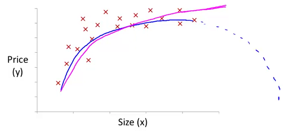
To make it a square root function, we could do: $h_\theta(x) = \theta_0 + \theta_1 x_1 + \theta_2 \sqrt{x_1}$
Note that at 2:52 and through 6:22 in the “Features and Polynomial Regression” video, the curve that Prof Ng discusses about “doesn’t ever come back down” is in reference to the hypothesis function that uses the
sqrt()function (shown by the solid purple line), not the one that uses $size^2$ (shown with the dotted blue line). The quadratic form of the hypothesis function would have the shape shown with the blue dotted line if $\theta _2$ was negative.
One important thing to keep in mind is, if you choose your features this way then feature scaling becomes very important.
- E.g. if $x_1$ has range $1 - 1000$ then range of $x^2_1$ becomes $1 - 1000000$ and that of $x^3_1$ becomes $1 - 1000000000$
- So you should scale $x_1$ before using polynomial regression.
Computing Parameters Analytically
Normal Equation
The “Normal Equation” (正规方程) is a method of finding the optimum $\theta$ without iteration.
There is no need to do feature scaling with the normal equation.
Intuition
$\theta \in R^{n+1} , J(\theta _0, \theta _1, \dots , \theta\_m) = \frac{1}{2m} \sum ^m\_{i=1} \left( h_\theta (x^{(i)}) - y^{(i)} \right) ^2$- Set
$\frac{\partial }{\partial \theta _j} J(\theta ) = \cdots = 0$ (for every $j$), solve for $\theta _0, \theta _1, \dots , \theta _m$
Method
We have $m$ examples $(x^{(1)}, y^{(1)}), \dots , (x^{(m)}, y^{(m)})$ and $n$ features. (Note that $x^{(i)}_0 = 0$)
$$x^{(i)} = \begin{bmatrix}x^{(i)}_0 \\ x^{(i)}_1 \\ x^{(i)}_2 \\ \vdots \\ x^{(i)}_n \end{bmatrix}$$
And construct the $m \times (n+1)$ matrix $X$
$$X = \begin{bmatrix} (x^{(1)})^T \\ (x^{(2)})^T \\ \vdots \\ (x^{(m)})^T \end{bmatrix}$$
And the $m$-dimension vector $y$
$$y = \begin{bmatrix}y^{(i)} \\ y^{(i)} \\ y^{(i)} \\ \vdots \\ y^{(m)} \end{bmatrix}$$
Finally, we can get
$$ \theta = (X^T X)^{-1}X^T y $$
Example
Suppose you have the training in the table below:
| age ($x_1$) | height in cm ($x_2$) | weight in kg ($y$) |
|---|---|---|
| 4 | 89 | 16 |
| 9 | 124 | 28 |
| 5 | 103 | 20 |
You would like to predict a child’s weight as a function of his age and height with the model
$$weight = \theta _0 + \theta _1 age + \theta _2 height$$
Then you can construct $X$ and $y$
$$X = \begin{bmatrix} 1 & 4 & 89 \\ 1 & 9 & 124 \\ 1 & 5 & 103 \end{bmatrix}$$
$$Y = \begin{bmatrix} 16 \\ 28 \\ 20 \end{bmatrix}$$
Usage in Octave
|
|
Comparison of gradient descent and the normal equation
$m$ training examples and $n$ features.
| Gradient Descent | Normal Equation |
|---|---|
| Need to choose $\alpha$ | No need to choose $\alpha$ |
| Needs many iterations | No need to iterate |
| $O (kn^2)$ | $O (n^3)$, need to calculate $(X^TX)^{-1}$ |
| Works well when $n$ is large | Slow if $n$ is very large |
With the normal equation, computing the inversion has complexity $O(n^3)$. So if we have a very large number of features, the normal equation will be slow. In practice, when $n$ exceeds 10,000 it might be a good time to go from a normal solution to an iterative process.
Normal Equation Noninvertibility
$$ \theta = (X^T X)^{-1}X^T y $$
- What if $X^TX$ is non-invertible (不可逆的) ? (singular/ degenerate)
- Octave:
pinv(X'*X)*X"*y- There’s two functions in Octave for inverting matrices,
pinv(pseudo-inverse, 伪逆) andinv(inverse). - As long as you use the
pinvfunction then this will actually compute the value of data that you want even if X transpose X is non-invertible. - So when implementing the normal equation in octave we want to use the
pinvfunction rather thaninv.
- There’s two functions in Octave for inverting matrices,
- $X^TX$ may be noninvertible. The common causes are:
- Redundant features, where two features are very closely related (i.e. they are linearly dependent)
- E.g. $x_1$ = size in $feet^2$, and $x_2$ = size in $m^2$. So you’ll always have $x_1 = (3.28)^2 x_2$
- Too many features (e.g. $m\le n$).
- In this case, delete some features or use “regularization”.
Octave/Matlab Tutorial
Basic Operations
- Print specific decimals:
disp(sprintf('6 decimals: %0.6f', a)) // 6 decimals: 3.141593 v = 1:0.2:2 // [1.0 1.2 1.4 1.6 1.8 2.0]ones,zeros,rand,randn(生成正态分布的随机数矩阵),eye(生成单位矩阵)hist(直方图,第二个参数课自定义条数)size(返回矩阵的行数与列数 [m n] )length(返回向量的维数)
Moving Data Around
- Use
loadto load data set.
|
|
Use
whoto show all variables in Octave workspacewhosfor detail informationclearto delete a variable
1clear featureXGet first ten elements of a matrix
|
|
- Use
saveto save your variable
|
|
By default the data is saved in binary. You can save it to ASCII by
1save hello.txt v -asciiUse
A(3, 2)to get $A_{32}$, orA(2, :)to get every element along the second rowA([1, 3], :)to get everything in the first and third rowsA(:, 2) = [10; 11; 12]to change the value of elements in second column.A = [A, [100; 101; 102]]to append another column vector to rightA(:)to put all elements of $A$ into a single vector
Computing on Data
- Use
maxto get the largest element in a vector
1 2 |
a = [1 15 2 0.5]; [val, ind] = max(a); // val = 15, ind = 2 |
If you do
max(A), where $A$ is a matrix, what this does is this actually does the column wise maximum.1 2 3 4 5 6 7 8
A = [1 2; 3 4; 5 6]; max(A) // [5 6] A = [8 1 6; 3 5 7; 4 9 2]; max(A, [], 1) // [8 9 7] (get the column wise maximum) max(A, [], 2) // [8 7 9] (get the row wise maximum) max(max(A)) // 9 max(A(:)) // 9
a < 3does the element wise operation, you’ll get[1 0 1 1]find(a<3)gets[1 3 4]
magic(3)gets a 3x3 magic matrixsum,prod,floor,ceil,flipud
Plotting Data
plothold on,figure,subplotxlabel,ylabel,legend,title,axisprint -dpng 'myPlot.png'imagesc(A)to visualize a matriximagesc(A), colorer, colormap grayto be in gray scale.
Control Statements: for, while, if statement
Vectorization
Vectorization is the process of taking code that relies on loops and converting it into matrix operations. It is more efficient, more elegant, and more concise.
As an example, let’s compute our prediction from a hypothesis. Theta is the vector of fields for the hypothesis and x is a vector of variables.
With loops ($h_\theta (x) =\theta_0 x_0 + \theta_1 x_1 + \theta_2 x_2 + \cdots + \theta_n x_n$):
1 2 3 4 |
prediction = 0.0; for j = 1:n+1, prediction += theta(j) * x(j); end; |
With vectorization ($h_\theta (x) = \theta^T x$):
1
|
prediction = theta' * x; |