Notes for CS231n Neural Network
Contents
本文主要对于 CS231n 课程自带的 Lecture Notes 的一些补充与总结. 建议先看原版的 Lecture Notes或者可以看知乎专栏中的中文翻译:
另外, 本文主要根据讲课的 Slides 上的顺序来, 与 Lecture Notes 的顺序略有不同.
Lecture 5
Activation Functions
课程中主要讲了Sigmoid, tanh, ReLU, Leaky ReLU, Maxout 以及 ELU 这几种激活函数.
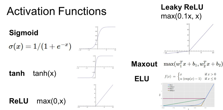
- Sigmoid 由于以下原因, 基本不使用
- 函数饱和使得梯度消失(Saturated neurons “kill” the gradients)
- 函数并非以零为中心(zero-centered)
- 指数运算消耗大量计算资源
- tanh 相对于 Sigmoid 来说, 多了零中心这一个特性, 但还是不常用
- 重头戏 ReLU (Rectified Linear Unit):
- 在正半轴上没有饱和现象
- 线性结构省下了很多计算资源, 可以直接对矩阵进行阈值计算来实现, 速度是 sigmoid/tanh 的6倍
- 然而由于负半轴直接是0, 训练的时候会”死掉”(die), 因此就有了 Leaky ReLU 和 ELU (Exponential Linear Units), 以及更加通用的 Maxout (代价是消耗两倍的计算资源)
实践中一般就直接选 ReLU, 同时注意 Learning Rate 的调整. 实在不行用 Leaky ReLU 或者 Mahout 碰碰运气. 还可以试试 tanh. 坚决别用 Sigmoid.
Data Preprocessing
有很多数据预处理的方法, 比如零中心化(zero-centering), 归一化(normalization), PCA(Principal Component Analysis, 主成分分析)和白化(Whitening).
- 零中心化(zero-centering): 主要方法就是均值减法, 将数据的中心移到原点上
|
|
零中心化主要有两种做法(e.g. consider CIFAR-10 example with [32,32,3] images):
Subtract the mean image (e.g.AlexNet) (mean image = [32,32,3] array)
Subtract per-channel mean (e.g.VGGNet) (mean along each channel = 3 numbers)
归一化(normalization): 使得数据所有维度的范围基本相等, 当然由于图像像素的数值范围本身基本是一致的(一般为0-255), 所以不一定要用.
|
|
- PCA 和白化在 CNN 中并没有什么用, 就不介绍了.
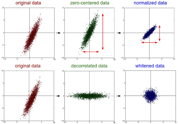
实践中一般就只做零中心化, 其他几样基本都不用做.
以下引自知乎专栏[智能单元]所翻译的课程讲义:
常见错误。进行预处理很重要的一点是:任何预处理策略(比如数据均值)都只能在训练集数据上进行计算,算法训练完毕后再应用到验证集或者测试集上。例如,如果先计算整个数据集图像的平均值然后每张图片都减去平均值,最后将整个数据集分成训练/验证/测试集,那么这个做法是错误的。应该怎么做呢?应该先分成训练/验证/测试集,只是从训练集中求图片平均值,然后各个集(训练/验证/测试集)中的图像再减去这个平均值。
译者注:此处确为初学者常见错误,请务必注意!
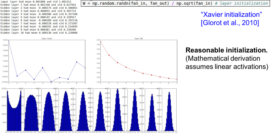
Weight Initialization
由于各种原因, 将 Weight 全部初始化为0, 或者是小随机数的方法都不大好(一个是由于对称性, 另一个是由于梯度信号太小). 建议使用的是下面这个(配合 ReLU):
|
|
或者 Xavier initialization:
另外就是还推荐 Batch Normalization (批量归一化), 通常应用在全连接层之后, 激活函数之前. 具体参见论文[Ioffe and Szegedy, 2015].
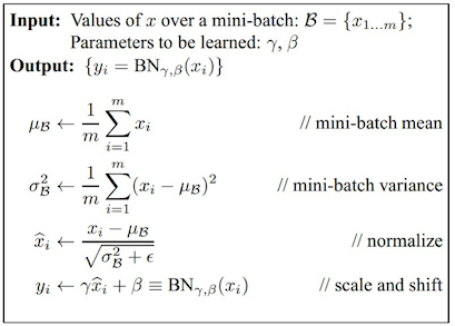
- Improves gradient flow through thenetwork
- Allows higher learning rates
- Reduces the strong dependence on initialization
- Acts as a form of regularization in afunny way, and slightly reduces the need for dropout, maybe
Babysitting the Learning Process
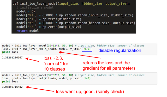
Double check that the loss is reasonable
- 首先不使用 regularization, 观察 loss 是否合理(下例中对于 CIFAR-10 的初始 loss 应近似等于$log(0.1)=2.31$)
- 然后再开启 regularization, 观察 loss 是否上升
Other sanity check tips
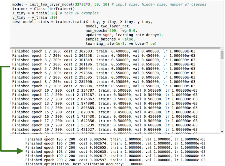
- 首先在一个小数据集上进行训练(可先设 regualrization 为0), 看看是否过拟合, 确保算法的正确性.
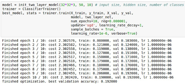
之后再从一个小的 regularization 开始, 寻找合适的能够使 loss 下降的 learning rate.
- 如果几次 epoch 后, loss 没没有下降, 说明 learning rate 太小了
- 如果 loss 爆炸了, 那么说明 learning rate 太大了
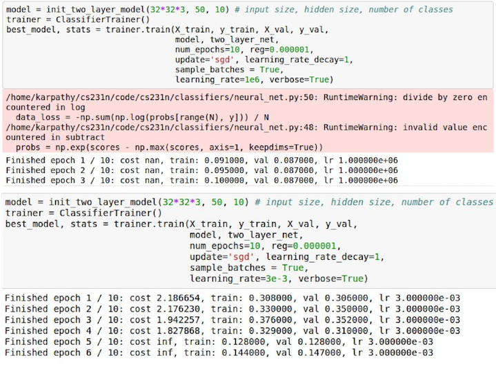
- 通常 learning rate 的范围是$[1e-3, 1e-5]$
Hyperparameter Optimization
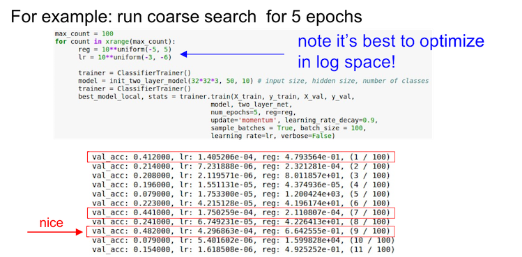
从粗放(coarse)到细致(fine)地分段搜索, 先大范围小周期(1-5 epoch足矣), 然后再根据结果小范围长周期
- First stage: only a few epochs to get rough idea of what params work
- Second stage: longer running time, finer search
- … (repeat as necessary)
If the cost is ever > 3 * original cost, break out early
在对数尺度上进行搜索, 例如
learning_rate = 10 ** uniform(-6, 1). 当然有些超参数还是按原来的, 比如dropout = uniform(0,1)小心边界上的最优值, 否则可能会错过更好的参数搜索范围.
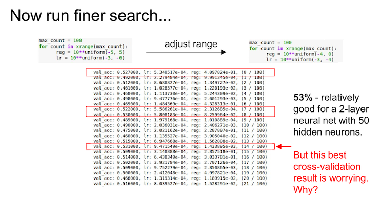
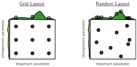
- 随机搜索优于网格搜索
Lecture 6
Parameter Updates
参数更新有很多种方法, 常见的如下图:
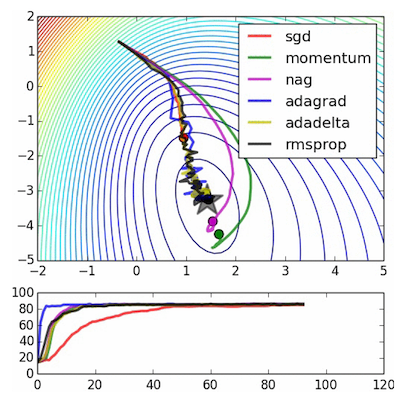
- 最普通的就是SGD, 仅仅按照负梯度来更新
|
|

- 其次就是各种动量方法, 比如 Momentum, 以及其衍生的 Nesterov 方法. 其主要思想就是在任何具有持续梯度的方向上保持一个会慢慢消失的动量, 使得梯度下降更为圆滑.
|
|
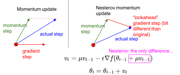
- v 初始为 0
- mu 一般取 0.5, 0.9 或 0.99. 有时候可以先 0.5, 然后慢慢变成 0.99
- 然后就是逐步改 learning rate 的方法, 比如 AdaGrad 或者 RMSProp (Hinton 大神在 Coursera 课上提出的改进方法)
|
|
- cache 尺寸与 dx 相同
- eps 取值在 1e-4 到 1e-8 之间, 主要是为了防止分母为 0.
- AdaGrad 通常过早停止学习, RMSProp 通过引入一个梯度平方的滑动平均改善了它.
- 最后就是集上述方法之大成的 Adam, 在大多数的实践中都是一个很好的选择.
|
|
- The bias correction compensates for the fact that m,v are initialized at zero and need some time to “warm up”. Only relevant in first few iterations when t is small.
Learning rate decay
主要是为了让 learning rate 随着训练时间的推移慢慢变小, 防止系统动能太大, 到最后在最优点旁边跳来跳去.
- step decay: e.g. decay learning rate by half every few epochs.
- exponential decay: $\alpha = \alpha_0 e^{-kt}$
- 1/t decay: $\alpha = \alpha_0 / (1+kt)$
Second order optimization methods
主要是一些基于牛顿法的二阶最优化方法, 包括 L-BGFS 之类的. 其优点是根本就没有 learning rate 这个超参数, 而缺点则是 Hessian 矩阵实在是太大了, 非常耗费时间与空间, 因此在 DL 和 CNN 中基本不使用.
Evaluation: Model Ensembles
训练多个独立的模型, 然后在测试的时候对其结果进行平均, 一般能得到 2% 的额外性能提升;
平均单个模型的多个记录点 (check point) 上的参数, 也能获得一些提升
训练的时候对参数进行平滑操作, 并用于测试集 (keep track of (and use at test time) a running average
parameter vector)
|
|
Regularization (dropout)
Dropout 算是很常用的一种方法了, 主要就是在前向传播的时候随机设置某些神经元为零 (“randomly set some neurons to zero in the forward pass”).
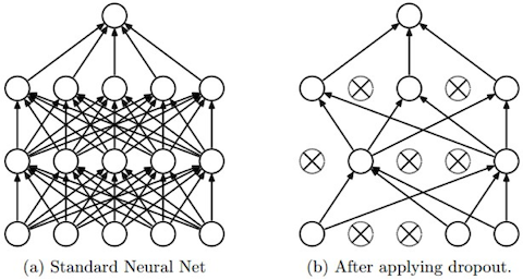
其主要想法是让网络具有一定的冗余能力 (Forces the network to have a redundant representation), 或者说是训练出了一个大的集成网络 (Dropout is training a large ensemble of models (that share parameters), each binary mask is one model, gets trained on only ~one datapoint.)
具体实现如下
|
|
Gradient Checking
主要就是通过数值法计算梯度, 然后和通过后向传播得到的解析梯度比较, 看看误差大不大, 防止手贱算错梯度导致后面算法全乱了.
- 用中心化公式$\frac{df(x)}{dx} = \frac{f(x+h - f(x-h)}{2h}$计算数值梯度, $h$取 $1e-5$ 左右.
- 使用相对误差$\frac{|f^{‘}_a - f^{‘}_n|}{max(|f^{‘}_a|, |f^{‘}_n|)}$
同时还有些注意事项, 参见 Gradient Checks.