从 RNN 开始, CS231n 的 Lecture Notes 就没有了, 因此我根据上课时的 Slides 整理了一些需要重视的知识点. 还可以参考这些文章或是视频来加深理解。

Lecture 10

Introduction

Recurrent Networks offer a lot of flexibility:

RNN_flexibility

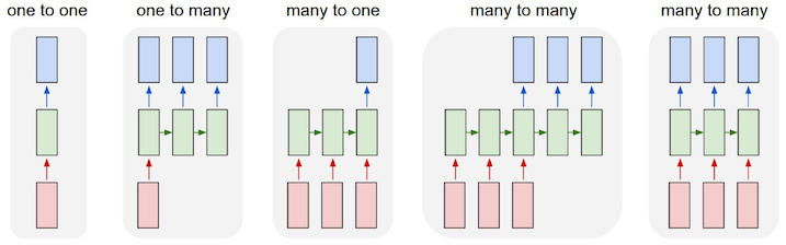
one to one: Vanilla Neural Networks
one to many: e.g. Image Captioning (image -> sequence of words)
many to one: e.g. Sentiment Classification (sequence of words -> sentiment)
many to many:
- e.g. Machine Translation (seq of words -> seq of words)
- e.g. Video classification on frame level

RNN can also do sequential precessing of fix inputs (Multiple Object Recognition with Visual Attention, Ba et al.) or fixed outputs (DRAW: A Recurrent Neural Network For Image Generation, Gregor et al.).

Recurrent Neural Network

Concept

Usually we want to predict a vector at some time steps. To achieve this goal, we can process a sequence of vectors $x$ by applying a recurrence formula at every time step:

RNN_concept

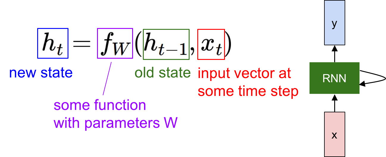
Notice: the same function and the same set of parameters are used at every time step. That’s to say, we use shared weights.

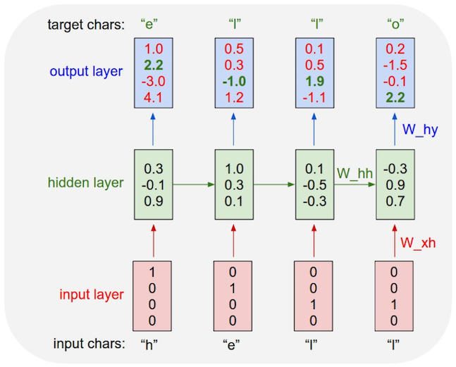
(Vanilla) Recurrent Neural Network

The state consists of a single “hidden” vector $h$:

$h_t = tanh (W_{hh} h_{t-1} + W_{xh} x_t)$
$y_t = W_{hy} h_t$

Example: Character-level language model

We have a vocabulary of four characters $\begin{bmatrix} h & e & l & o \end{bmatrix}$, and the example training sequence is “hello”.

character-level_language_model_example

And we can look its the implement.

Data I/O

 1
 2
 3
 4
 5
 6
 7
 8
 9
10
11
12
13


"""
Minimal character-level Vanilla RNN model. Written by Andrej Karpathy (@karpathy)
BSD License
"""
import numpy as np

# data I/O
data = open('input.txt', 'r').read() # should be simple plain text file
chars = list(set(data))
data_size, vocab_size = len(data), len(chars)
print 'data has %d characters, %d unique.' % (data_size, vocab_size)
char_to_ix = { ch:i for i,ch in enumerate(chars) }
ix_to_char = { i:ch for i,ch in enumerate(chars) }

Initializations

 1
 2
 3
 4
 5
 6
 7
 8
 9
10
11


# hyperparameters
hidden_size = 100 # size of hidden layer of neurons
seq_length = 25 # number of steps to unroll the RNN for
learning_rate = 1e-1

# model parameters
Wxh = np.random.randn(hidden_size, vocab_size)*0.01 # input to hidden
Whh = np.random.randn(hidden_size, hidden_size)*0.01 # hidden to hidden
Why = np.random.randn(vocab_size, hidden_size)*0.01 # hidden to output
bh = np.zeros((hidden_size, 1)) # hidden bias
by = np.zeros((vocab_size, 1)) # output bias

Main Loop

 1
 2
 3
 4
 5
 6
 7
 8
 9
10
11
12
13
14
15
16
17
18
19
20
21
22
23
24
25
26
27
28
29
30
31
32


n, p = 0, 0
mWxh, mWhh, mWhy = np.zeros_like(Wxh), np.zeros_like(Whh), np.zeros_like(Why)
mbh, mby = np.zeros_like(bh), np.zeros_like(by) # memory variables for Adagrad
smooth_loss = -np.log(1.0/vocab_size)*seq_length # loss at iteration 0
while True:
  # prepare inputs (we're sweeping from left to right in steps seq_length long)
  if p+seq_length+1 >= len(data) or n == 0:
    hprev = np.zeros((hidden_size,1)) # reset RNN memory
    p = 0 # go from start of data
  inputs = [char_to_ix[ch] for ch in data[p:p+seq_length]]
  targets = [char_to_ix[ch] for ch in data[p+1:p+seq_length+1]]

  # sample from the model now and then
  if n % 100 == 0:
    sample_ix = sample(hprev, inputs[0], 200)
    txt = ''.join(ix_to_char[ix] for ix in sample_ix)
    print '----\n %s \n----' % (txt, )

  # forward seq_length characters through the net and fetch gradient
  loss, dWxh, dWhh, dWhy, dbh, dby, hprev = lossFun(inputs, targets, hprev)
  smooth_loss = smooth_loss * 0.999 + loss * 0.001
  if n % 100 == 0: print 'iter %d, loss: %f' % (n, smooth_loss) # print progress

  # perform parameter update with Adagrad
  for param, dparam, mem in zip([Wxh, Whh, Why, bh, by],
                                [dWxh, dWhh, dWhy, dbh, dby],
                                [mWxh, mWhh, mWhy, mbh, mby]):
    mem += dparam * dparam
    param += -learning_rate * dparam / np.sqrt(mem + 1e-8) # adagrad update

  p += seq_length # move data pointer
  n += 1 # iteration counter

Loss function

forward pass (compute loss)
backward pass (compute param gradient)

 1
 2
 3
 4
 5
 6
 7
 8
 9
10
11
12
13
14
15
16
17
18
19
20
21
22
23
24
25
26
27
28
29
30
31
32
33
34
35


def lossFun(inputs, targets, hprev):
  """
  inputs,targets are both list of integers.
  hprev is Hx1 array of initial hidden state
  returns the loss, gradients on model parameters, and last hidden state
  """
  xs, hs, ys, ps = {}, {}, {}, {}
  hs[-1] = np.copy(hprev)
  loss = 0
  # forward pass
  for t in xrange(len(inputs)):
    xs[t] = np.zeros((vocab_size,1)) # encode in 1-of-k representation
    xs[t][inputs[t]] = 1
    hs[t] = np.tanh(np.dot(Wxh, xs[t]) + np.dot(Whh, hs[t-1]) + bh) # hidden state
    ys[t] = np.dot(Why, hs[t]) + by # unnormalized log probabilities for next chars
    ps[t] = np.exp(ys[t]) / np.sum(np.exp(ys[t])) # probabilities for next chars
    loss += -np.log(ps[t][targets[t],0]) # softmax (cross-entropy loss)
  # backward pass: compute gradients going backwards
  dWxh, dWhh, dWhy = np.zeros_like(Wxh), np.zeros_like(Whh), np.zeros_like(Why)
  dbh, dby = np.zeros_like(bh), np.zeros_like(by)
  dhnext = np.zeros_like(hs[0])
  for t in reversed(xrange(len(inputs))):
    dy = np.copy(ps[t])
    dy[targets[t]] -= 1 # backprop into y. see http://cs231n.github.io/neural-networks-case-study/#grad if confused here
    dWhy += np.dot(dy, hs[t].T)
    dby += dy
    dh = np.dot(Why.T, dy) + dhnext # backprop into h
    dhraw = (1 - hs[t] * hs[t]) * dh # backprop through tanh nonlinearity
    dbh += dhraw
    dWxh += np.dot(dhraw, xs[t].T)
    dWhh += np.dot(dhraw, hs[t-1].T)
    dhnext = np.dot(Whh.T, dhraw)
  for dparam in [dWxh, dWhh, dWhy, dbh, dby]:
    np.clip(dparam, -5, 5, out=dparam) # clip to mitigate exploding gradients
  return loss, dWxh, dWhh, dWhy, dbh, dby, hs[len(inputs)-1]

Sampling

 1
 2
 3
 4
 5
 6
 7
 8
 9
10
11
12
13
14
15
16
17


def sample(h, seed_ix, n):
  """
  sample a sequence of integers from the model
  h is memory state, seed_ix is seed letter for first time step
  """
  x = np.zeros((vocab_size, 1))
  x[seed_ix] = 1
  ixes = []
  for t in xrange(n):
    h = np.tanh(np.dot(Wxh, x) + np.dot(Whh, h) + bh)
    y = np.dot(Why, h) + by
    p = np.exp(y) / np.sum(np.exp(y))
    ix = np.random.choice(range(vocab_size), p=p.ravel())
    x = np.zeros((vocab_size, 1))
    x[ix] = 1
    ixes.append(ix)
  return ixes

Gradient Check

 1
 2
 3
 4
 5
 6
 7
 8
 9
10
11
12
13
14
15
16
17
18
19
20
21
22
23
24
25
26


# gradient checking
from random import uniform
def gradCheck(inputs, target, hprev):
  global Wxh, Whh, Why, bh, by
  num_checks, delta = 10, 1e-5
  _, dWxh, dWhh, dWhy, dbh, dby, _ = lossFun(inputs, targets, hprev)
  for param,dparam,name in zip([Wxh, Whh, Why, bh, by], [dWxh, dWhh, dWhy, dbh, dby], ['Wxh', 'Whh', 'Why', 'bh', 'by']):
    s0 = dparam.shape
    s1 = param.shape
    assert s0 == s1, 'Error dims dont match: %s and %s.' % (`s0`, `s1`)
    print name
    for i in xrange(num_checks):
      ri = int(uniform(0,param.size))
      # evaluate cost at [x + delta] and [x - delta]
      old_val = param.flat[ri]
      param.flat[ri] = old_val + delta
      cg0, _, _, _, _, _, _ = lossFun(inputs, targets, hprev)
      param.flat[ri] = old_val - delta
      cg1, _, _, _, _, _, _ = lossFun(inputs, targets, hprev)
      param.flat[ri] = old_val # reset old value for this parameter
      # fetch both numerical and analytic gradient
      grad_analytic = dparam.flat[ri]
      grad_numerical = (cg0 - cg1) / ( 2 * delta )
      rel_error = abs(grad_analytic - grad_numerical) / abs(grad_numerical + grad_analytic)
      print '%f, %f => %e ' % (grad_numerical, grad_analytic, rel_error)
      # rel_error should be on order of 1e-7 or less

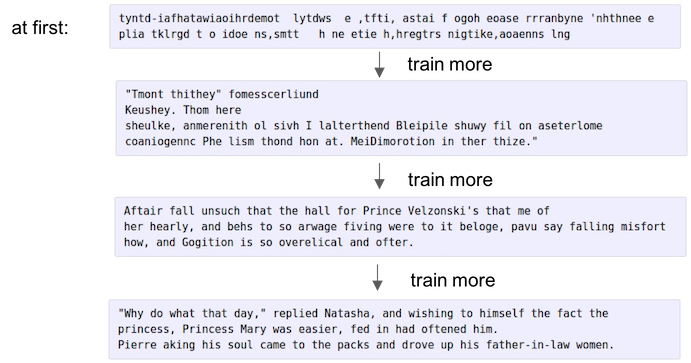
Results

Using Shakespeare’s sonnet as input:

RNN_text_generator

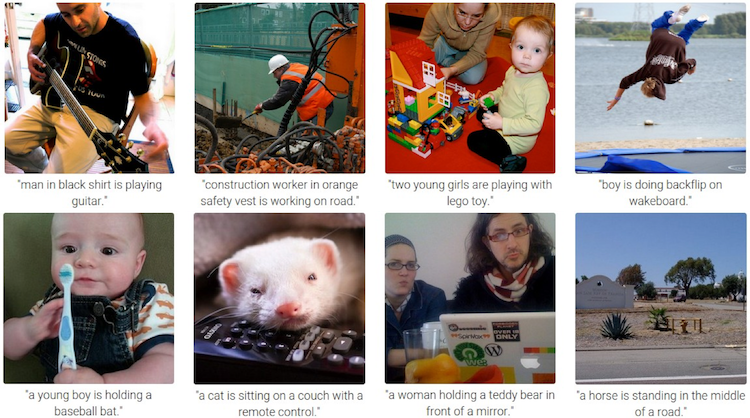
Example: Image Captioning

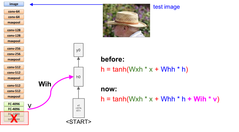
We use CNN to recognize objects and use RNN to generate captions.

image_captioning_structure

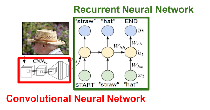
Cut the last two layers from CNN and connect it to RNN:

image_captioning_structure_1

And smaple the output from previous layer to next layer as input:

image_captioning_structure_2

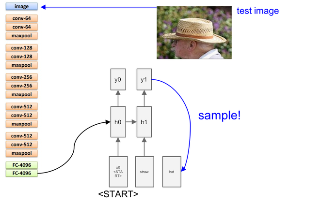
Sampling is stoped when meeting an END

image_captioning_structure_3

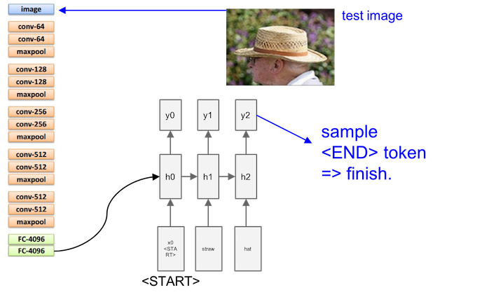
Finally, we’ll get a complete sentence (using Microsoft COCO dataset). The first row are good, but the second row may be not satisfactory.

image_captioning_result

Reference:

Explain Images with Multimodal Recurrent Neural Networks, Mao et al.

Deep Visual-Semantic Alignments for Generating Image Descriptions, Karpathy and Fei-Fei

Show and Tell: A Neural Image Caption Generator, Vinyals et al.

Long-term Recurrent Convolutional Networks for Visual Recognition andDescription, Donahue et al.

Learning a Recurrent Visual Representation for Image CaptionGeneration, Chen and Zitnick

More examples

We can also use RNN to generate open source textbooks written in LaTex, or generate C code from Linux source code, or searching for interpretable cells.

Long Short Term Memory (LSTM)

Vanishing/Exploding gradients

Exploding gradients
- Truncated BPTT
- Clip gradients at threshold (something like anti-windup in control science LOL)
- RMSProp to adjust learning rate
Vanishing gradients
- Harder to detect
- Weight Initialization
- ReLU activation functions
- RMSProp
- LSTM, GRUs (<– That’s why we use LSTM)

Introduction

LSTM is proposed in [Hochreiter et al., 1997]. GRU is a knid of simplified LSTM.

LSTM_diagram

ResNet is to PlainNet what LSTM is to RNN, kind of.

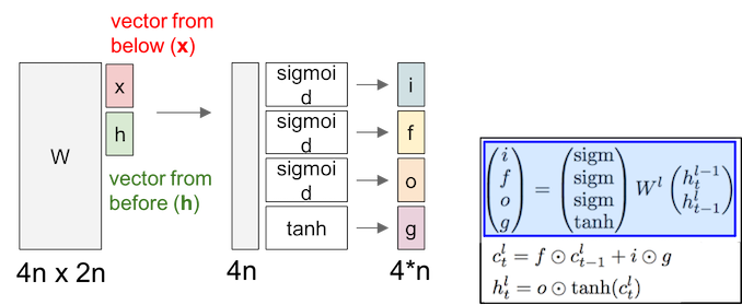
Concept

LSTM_structure

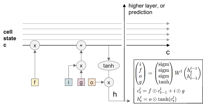
LSTM have two states, one is cell state ($c$), another is hidden state ($h$):

$i$: input gate, “add to memory”, decides whether do we want to add value to this cell.
$f$: forget gate, “flush the memory”, decides whether to shut off the cell and reset the counter.
$o$: output gate, “get from memory”, decides how much do we want to get from this cell.
$g$: input, decides how much do we want to add to this cell.

Summary

RNNs allow a lot of flexibility inarchitecture design
Vanilla RNNs are simple but don’twork very well
Common to use LSTM or GRU: theiradditive interactions improve gradient flow
Backward flow of gradients in RNNcan explode or vanish. Exploding is controlled with gradient clipping.Vanishing is controlled with additive interactions (LSTM)
Better/simpler architectures are ahot topic of current research
Better understanding (boththeoretical and empirical) is needed.

(To be improved by adding extra materials…)

Notes for CS231n Recurrent Neural Network

Contents

Lecture 10

Introduction

Recurrent Neural Network

Concept

Example: Character-level language model

Example: Image Captioning

More examples

Long Short Term Memory (LSTM)

Vanishing/Exploding gradients

Introduction

Concept

Summary

References