Notes for Machine Learning - Week 4
Contents
Neural Networks: Representation
Motivations
Non-linear Hypotheses
Performing linear regression with a complex set of data with many features is very unwieldy. For 100 features, if we wanted to make them quadratic we would get 5050 resulting new features.
We can approximate the growth of the number of new features we get with all quadratic terms with $\mathcal{O}(n^2/2)$. And if you wanted to include all cubic terms in your hypothesis, the features would grow asymptotically at $\mathcal{O}(n^3)$. These are very steep growths, so as the number of our features increase, the number of quadratic or cubic features increase very rapidly and becomes quickly impractical.
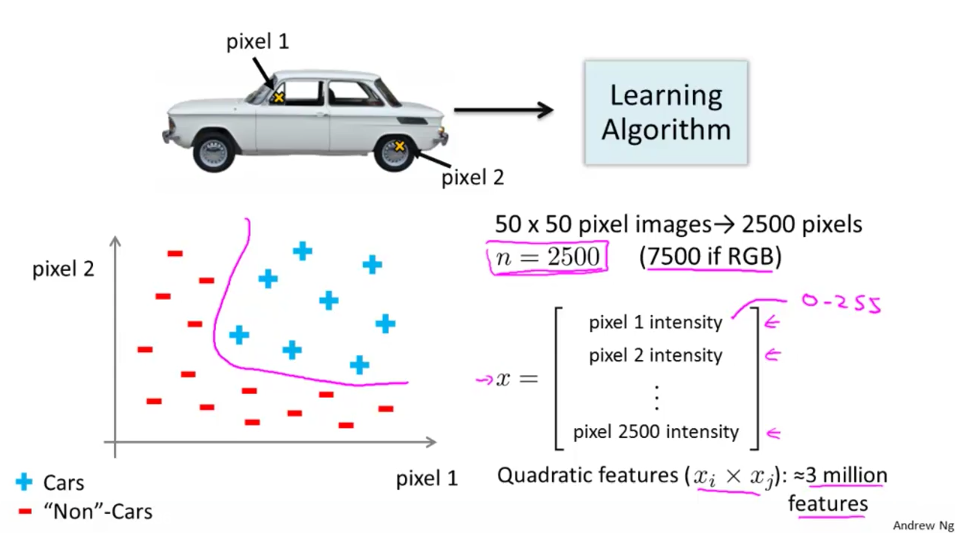
Example: let our training set be a collection of 50x50 pixel black-and-white photographs, and our goal will be to classify which ones are photos of cars. Our feature set size is then n=2500 if we compare every pair of pixels (7500 if RGB). Now let’s say we need to make a quadratic hypothesis function. With quadratic features, our growth is $\mathcal{O}(n^2⁄2)$. So our total features will be about 25002/2=3125000, which is very impractical.
Neurons and the Brain
Origins: Algorithms that try to mimic the brain.
- Was very widely used in 80s and early 90s; popularity diminished in late 90s.
- Recent resurgence: State-of-the-art technique for mant applications
The “one learning algorithm” hypothesis
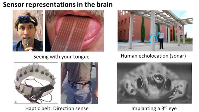
There is evidence that the brain uses only one “learning algorithm” for all its different functions. Scientists have tried cutting (in an animal brain) the connection between the ears and the auditory cortex and rewiring the optical nerve with the auditory cortex to find that the auditory cortex literally learns to see.

Neural Networks
Model Representation I
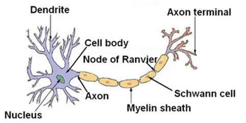
Neuron in the brain
At a very simple level, neurons are basically computational units that take input (dendrites, 树突) as electrical input (called “spikes”) that are channeled to outputs (axons, 轴突).
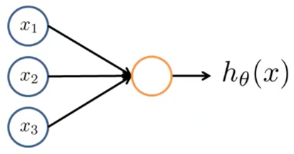
Neuron model: Logistic unit
- In our model, our dendrites are like the input features ($x_1 \cdots x_n$), and the output is the result of our hypothesis function $h_\theta (x)$:
- In this model our $x_0$ input node is sometimes called the “bias unit.” It is always equal to 1.
- In neural networks, we use the same logistic function as in classification: $\frac{1}{1 + e^{-\theta^Tx}}$. In neural networks however we sometimes call it a sigmoid (logistic) activation function.
- Our $\theta$ parameters are sometimes instead called “weights” in the neural networks model.
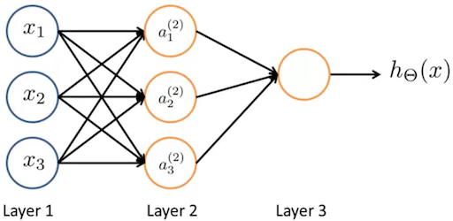
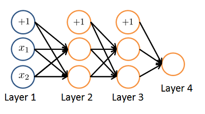
Neural Network
- The first layer is called the “input layer” and the final layer the “output layer”, which gives the final value computed on the hypothesis.
- We can have intermediate layers of nodes between the input and output layers called the “hidden layer”.
- $a_i^{(j)}$ = “activation” of unit $i$ in layer $j$
- $a_1^{(2)} = g(\Theta_{10}^{(1)}x_0 + \Theta_{11}^{(1)}x_1 + \Theta_{12}^{(1)}x_2 + \Theta_{13}^{(1)}x_3)$
- $a_2^{(2)} = g(\Theta_{20}^{(1)}x_0 + \Theta_{21}^{(1)}x_1 + \Theta_{22}^{(1)}x_2 + \Theta_{23}^{(1)}x_3)$
- $a_3^{(2)} = g(\Theta_{30}^{(1)}x_0 + \Theta_{31}^{(1)}x_1 + \Theta_{32}^{(1)}x_2 + \Theta_{33}^{(1)}x_3)$
- $h_\Theta(x) = a_1^{(3)} = g(\Theta_{10}^{(2)}a_0^{(2)} + \Theta_{11}^{(2)}a_1^{(2)} + \Theta_{12}^{(2)}a_2^{(2)} + \Theta_{13}^{(2)}a_3^{(2)})$
- $\Theta^{(j)}$ = matrix of weights controlling function mapping from layer $j$ to layer $j+1$
- If network has
$s_j$units in layer $j$ and$s_{j+1}$units in layer $j+1$, then$\Theta ^{(j)}$will be of dimension$s_{j+1}×(s_{j}+1)$.
- If network has
Model Representation II
Forward propagation: Vectorized implementation
The vector representation of $x$ and $z^{(j)}$ is:
$x = \begin{bmatrix}x_0 \\ x_1 \\ \cdots \\ x_n\end{bmatrix} , z^{(j)} = \begin{bmatrix}z_1^{(j)} \\ z_2^{(j)} \\ \cdots \\ z_n^{(j)}\end{bmatrix}$
Setting $x=a^{(1)}$, we can rewrite the equation as:
$z^{(j)} = \Theta^{(j-1)}a^{(j-1)}$
Now we can get a vector of our activation nodes for layer $j$ as follows:
$a^{(j)} = g(z^{(j)})$
We can then add a bias unit (equal to 1) to layer $j$ after we have computed $a^{(j)}$. This will be element $a^{(j)}_0$ and will be equal to 1.
We then get our final result with:
$h_\Theta(x) = a^{(j+1)} = g(z^{(j+1)})$
This last theta matrix ($\Theta ^{(j)}$) will have only one row so that our result is a single number.
All of this is called Forward propagation (前向传播). The forward propagation step in a neural network works where you start from the activations of the input layer and forward propagate that to the first hidden layer, then the second hidden layer, and then finally the output layer.
Neural Network learning its own features
The neural network, instead of being constrained to feed the features $x_1$, $x_2$, $x_3$ to logistic regression. It gets to learn its own features, $a_1$, $a_2$, $a_3$, to feed into the logistic regression.
Depending on what parameters it chooses for $\Theta _1$, you can learn some pretty interesting and complex features and therefore you can end up with a better hypotheses than using the raw features.
Applications
Examples and Intuitions I
AND function
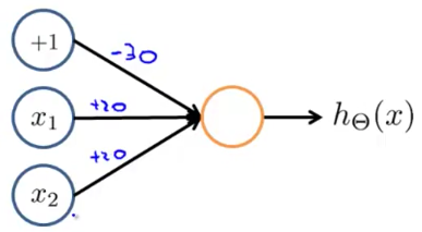
We have:
- $x_1, x_2 \in {0,1}$
- $y=x_1\ AND\ x_2$
- $\Theta^{(1)} =\begin{bmatrix}-30 & 20 & 20\end{bmatrix}$
And we know the plot of sigmoid function
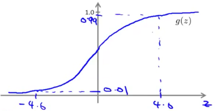
So the results of $h_\Theta(x) = g(-30 + 20x_1 + 20x_2)$ are
| $x_1$ | $x_2$ | $h_\Theta (x)$ |
|---|---|---|
| 0 | 0 | $g(-30) \approx 0$ |
| 0 | 1 | $g(-10) \approx 0$ |
| 1 | 0 | $g(-10) \approx 0$ |
| 1 | 1 | $g(10) \approx 1$ |
OR function
$\Theta^{(1)} =\begin{bmatrix}-10 & 20 & 20\end{bmatrix}$
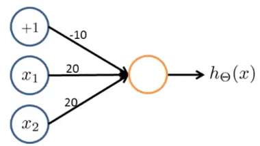
| $x_1$ | $x_2$ | $h_\Theta (x)$ |
|---|---|---|
| 0 | 0 | $g(-10) \approx 0$ |
| 0 | 1 | $g(10) \approx 1$ |
| 1 | 0 | $g(10) \approx 1$ |
| 1 | 1 | $g(10) \approx 1$ |
Examples and Intuitions II
Negation (NOT function)
$\Theta^{(1)} =\begin{bmatrix}10 & -20\end{bmatrix}$
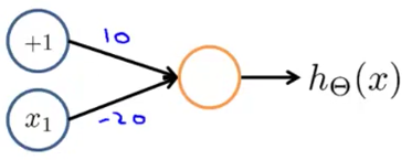
| $x_1$ | $h_\Theta (x)$ |
|---|---|
| 0 | $g(10) \approx 1$ |
| 1 | $g(-10) \approx 0$ |
NOR function
$\Theta^{(1)} = \begin{bmatrix}10 & -20 & -20\end{bmatrix}$
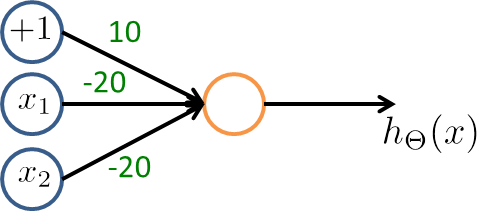
| $x_1$ | $x_2$ | $h_\Theta (x)$ |
|---|---|---|
| 0 | 0 | $g(10) \approx 1$ |
| 0 | 1 | $g(-10) \approx 0$ |
| 1 | 0 | $g(-10) \approx 0$ |
| 1 | 1 | $g(-30) \approx 0$ |
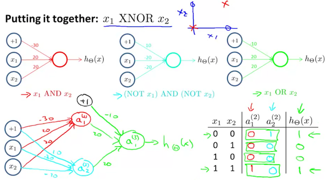
XNOR function
Multiclass Classification
To classify data into multiple classes, we let our hypothesis function return a vector of values. Say we wanted to classify our data into one of four final resulting classes:
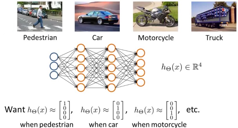
Our final layer of nodes, when multiplied by its theta matrix, will result in another vector, on which we will apply the $g()$ logistic function to get a vector of hypothesis values.
Our resulting hypothesis for one set of inputs may look like:
$h_\Theta(x) = \begin{bmatrix}0 \\ 0 \\ 1 \\ 0 \\ \end{bmatrix}$
In which case our resulting class is the third one down, or $h_\Theta (x)_3$.
We can define our set of resulting classes as $y$:
$y^{(i)} = \begin{bmatrix}1\\ 0\\ 0\\ 0\end{bmatrix},\ \begin{bmatrix}0 \\ 1\\ 0\\ 0\end{bmatrix},\ \begin{bmatrix}0\\ 0\\ 1\\ 0\end{bmatrix},\ \begin{bmatrix}0\\ 0\\ 0\\ 1\end{bmatrix}$
Our final value of our hypothesis for a set of inputs will be one of the elements in $y$.
Quiz
Which of the following statements are true? Check all that apply.
- TRUE If a neural network is overfitting the data, one solution would be to increase the regularization parameter $\lambda$.
- FALSE If a neural network is overfitting the data, one solution would be to decrease the regularization parameter $\lambda$.
- FALSE Suppose you have a multi-class classification problem with three classes, trained with a 3 layer network. Let $a^{(3)}_1 = (h_\Theta(x))_1$ be the activation of the first output unit, and similarly $a^{(3)}_2 = (h_\Theta(x))_2$ and $a^{(3)}_3 = (h_\Theta(x))_3$. Then for any input x, it must be the case that $a^{(3)}_1 + a^{(3)}_2 + a^{(3)}_3 = 1$.
- The outputs of a neural network are not probabilities, so their sum need not be 1.
- TRUE In a neural network with many layers, we think of each successive layer as being able to use the earlier layers as features, so as to be able to compute increasingly complex functions.
Consider the following neural network which takes two binary-valued inputs $x_1,x_2\in {0,1}$ and outputs $h_\Theta (x)$. Which of the following logical functions does it (approximately) compute?
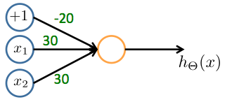
- OR
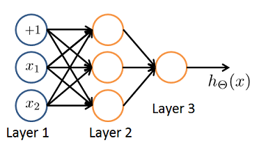
- Consider the neural network given below. Which of the following equations correctly computes the activation $a{(3)}_1$? Note: $g(z)$ is the sigmoid activation function.
- $a_1^{(3)} = g(\Theta_{1,0}^{(2)}a_0^{(2)} + \Theta_{1,1}^{(2)}a_1^{(2)} + \Theta_{1,2}^{(2)}a_2^{(2)})$
- You have the following neural network:
You’d like to compute the activations of the hidden layer $a^{(2)}\in R^3$. One way to do so is the following Octave code:
|
|
You want to have a vectorized implementation of this (i.e., one that does not use for loops). Which of the following implementations correctly compute $a^{(2)}$? Check all that apply.
a2 = sigmoid (Theta1 * x);
- You are using the neural network pictured below and have learned the parameters $\Theta^{(1)} = \begin{bmatrix} 1 & 0.5 & 1.9 \\ 1 & 1.2 & 2.7 \end{bmatrix}$ and $\Theta^{(2)} = \begin{bmatrix} 1 & -0.2 & -1.7 \end{bmatrix}$. Suppose you swap the parameters for the first hidden layer between its two units so $\Theta^{(1)} = \begin{bmatrix} 1 & 1.2 & 2.7 \\ 1 & 0.5 & 1.9 \end{bmatrix}$ and also swap the output layer so $\Theta^{(2)} = \begin{bmatrix} 1 & -1.7 & -0.2 \end{bmatrix}$. How will this change the value of the output $h_\Theta (x)$?
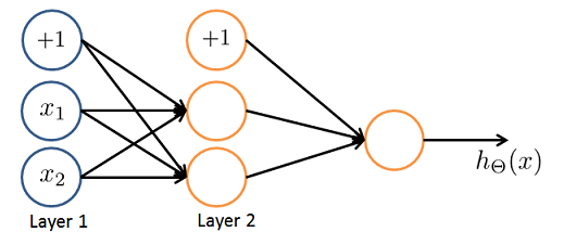
- It will stay the same.