Neural Networks: Learning

Cost Function and Backpropagation

Cost Function

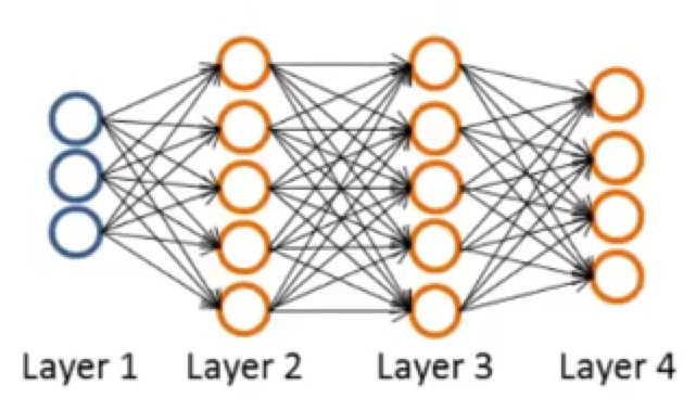
Let’s first define a few variables that we will need to use:

• $L$ = total number of layers in the network
• $s_l$ = number of units (not counting bias unit) in layer $l$
• $K$ = number of output units/classes

Recall that the cost function for regularized logistic regression was:

$J(\theta) = - \frac{1}{m} \sum_{i=1}^m \large[ y^{(i)}\ \log (h_\theta (x^{(i)})) + (1 - y^{(i)})\ \log (1 - h_\theta(x^{(i)}))\large] + \frac{\lambda}{2m}\sum_{j=1}^n \theta_j^2$

For neural networks, it is going to be slightly more complicated:

$J(\Theta) = - \frac{1}{m} \sum_{i=1}^m \sum_{k=1}^K \left[y^{(i)}_k \log ((h_\Theta (x^{(i)}))_k) + (1 - y^{(i)}_k)\log (1 - (h_\Theta(x^{(i)}))_k)\right] + \frac{\lambda}{2m}\sum_{l=1}^{L-1} \sum_{i=1}^{s_l} \sum_{j=1}^{s_{l+1}} ( \Theta_{j,i}^{(l)})^2$

• $h_\Theta (x) \in R^K$, $(h_\Theta (x))_i$ = $i^{th}$ output
• In the first part of the equation, the double sum simply adds up the logistic regression costs calculated for each cell in the output layer
• In the regularization part, the triple sum simply adds up the squares of all the individual $\Theta$s in the entire network.
  • The number of columns in our current theta matrix is equal to the number of nodes in our current layer (including the bias unit).
  • The number of rows in our current theta matrix is equal to the number of nodes in the next layer (excluding the bias unit).
  • This is like a bias unit and by analogy to what we were doing for logistic progression, we won’t sum over those terms in our regularization term because we don’t want to regularize them and string their values as zero.

Backpropagation Algorithm

“Backpropagation” (后向搜索) is neural-network terminology for minimizing our cost function, just like what we were doing with gradient descent in logistic and linear regression.

Our goal is try to find parameters $\Theta$ to try to minimize $J(\Theta)$.

In order to use either gradient descent or one of the advance optimization algorithms. What we need to do therefore is to write code that takes this input the parameters theta and computes $J(\Theta)$ and $\dfrac{\partial}{\partial \Theta_{i,j}^{(l)}}J(\Theta)$.

Gradient compuation

Given one training example $(x,y)$

Forward propagation:

• $a^{(1)} = x$
• $z^{(2)} = \Theta ^{(1)} a ^{(1)}$
• $a^{(2)} = g(z^{(2)})\ (add\ a^{(2)}_0)$
• $z^{(3)} = \Theta ^{(1)} a ^{(2)}$
• $a^{(3)} = g(z^{(3)})\ (add\ a^{(3)}_0)$
• $z^{(4)} = \Theta ^{(3)} a ^{(3)}$
• $a^{(2)} = h_\Theta (x) = g(z^{(3)})$

In backpropagation we’re going to compute for every node:

$\delta_j^{(l)}$ = “error” of node j in layer $l$ ($s_{l+1}$ elements vector)

For each output unit (layer $L = 4$):

$\delta ^{(4)} = a^{(4)} - y$

To get the delta values of the layers before the last layer, we can use an equation that steps us back from right to left:

$\delta^{(l)} = ((\Theta^{(l)})^T \delta^{(l+1)})\ .*\ g’(z^{(l)})$

The g-prime derivative terms can also be written out as:

$g’(z^{(l)}) = a^{(l)}\ .*\ (1 - a^{(l)})$

There is no $\delta ^{(1)}$ term, because the first layer corresponds to the input layer and that’s just the feature we observed in our training sets, so that doesn’t have any error associated with that.

It’s possible to prove that if you ignore regularation, then the partial derivative terms you want are exactly given by the activations and these delta terms.

$\dfrac{\partial J(\Theta)}{\partial \Theta_{i,j}^{(l)}} = a^{(i)}_j \delta^{(l+1)}_i\ (\text{ignoring }\lambda)$

Backpropagation Algorithm

• Training set $\lbrace (x^{(1)}, y^{(1)}) \cdots (x^{(m)}, y^{(m)})\rbrace$
• Set $\Delta^{(l)}_{i,j} := 0$ (for all $l, i, j$)
• For $i=1$ to $m$
  • Set $a^{(1)} := x^{(t)}$
  • Perform forward propagation to compute $a^{(l)}$ for $l = 2,3,\dots ,L$
  • Using $y^{(i)}$, compute $\delta^{(L)} = a^{(L)} - y^{(t)}$
  • Compute $\delta^{(L-1)}, \delta^{(L-2)},\dots,\delta^{(2)}$
  • $\Delta^{(l)}_{i,j} := \Delta^{(l)}_{i,j} + a_j^{(l)} \delta_i^{(l+1)}$  or with vectorization, $\Delta^{(l)} := \Delta^{(l)} + \delta^{(l+1)}(a^{(l)})^T$
• $D^{(l)}_{i,j} := \dfrac{1}{m}\left(\Delta^{(l)}_{i,j} + \lambda\Theta^{(l)}_{i,j}\right)$ If $j\ne 0$ 
• $D^{(l)}_{i,j} := \dfrac{1}{m}\Delta^{(l)}_{i,j}$ If $j = 0$

The capital-delta matrix is used as an “accumulator” to add up our values as we go along and eventually compute our partial derivative.

 the $D_{i,j}^{(l)}$ terms are the partial derivatives and the results we are looking for:

$\dfrac{\partial J(\Theta)}{\partial \Theta_{i,j}^{(l)}} = D_{i,j}^{(l)}$

Backpropagation Intuition

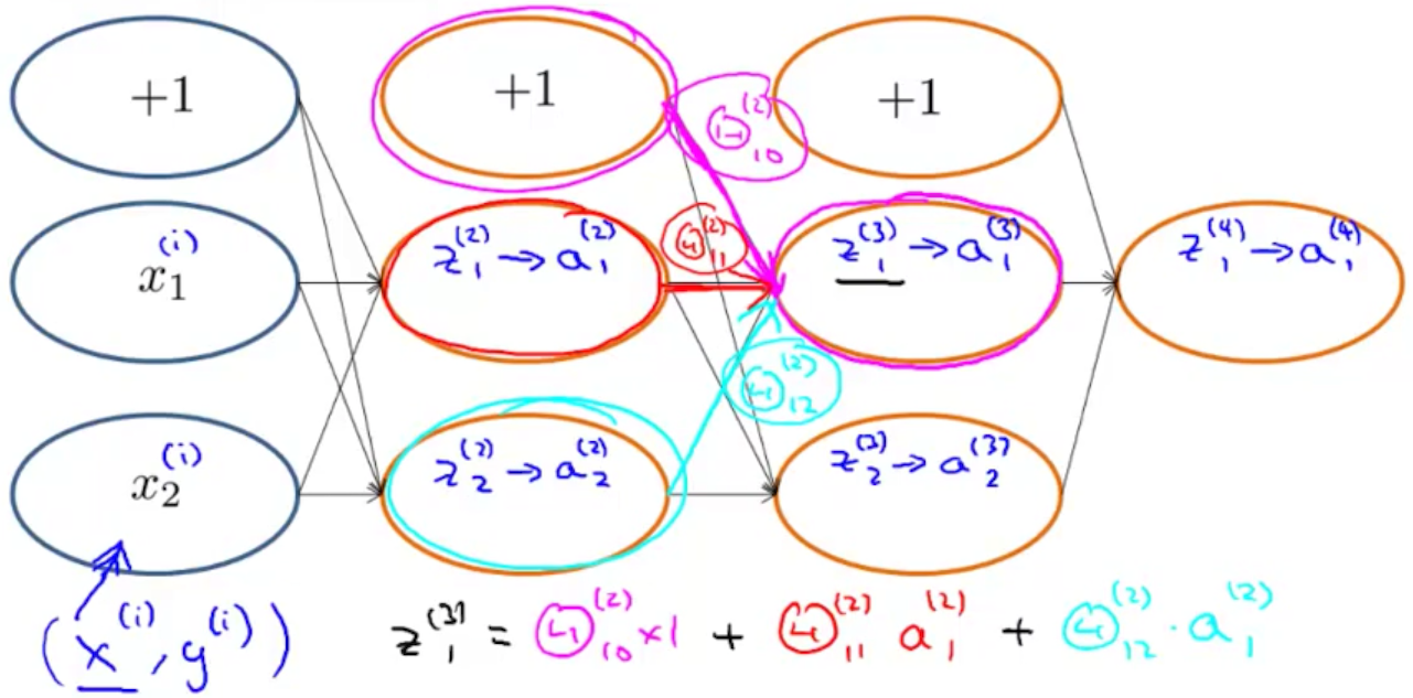
Forward propagation

What’s backpropagation doing?

The cost function is:

$J(\theta) = - \frac{1}{m} \sum_{t=1}^m\sum_{k=1}^K \left[ y^{(t)}_k \ \log (h_\theta (x^{(t)}))_k + (1 - y^{(t)}_k)\ \log (1 - h_\theta(x^{(t)})_k)\right] + \frac{\lambda}{2m}\sum_{l=1}^{L-1} \sum_{i=1}^{s_l} \sum_{j=1}^{s_l+1} ( \theta_{j,i}^{(l)})^2$

Focusing on a single example $x^{(i)}, y^{(i)}$, the case of 1 output unit, and ignoring regularization ($\lambda = 0$),

$cost(t) =y^{(t)} \ \log (h_\theta (x^{(t)})) + (1 - y^{(t)})\ \log (1 - h_\theta(x^{(t)}))$

Intuitively, $\theta ^{(l)}_j$ is the “error” for $a ^{(l)}_j$ (unit $j$ in layer $l$). More formally, the delta values are actually the derivative of the cost function:

$\delta_j^{(l)} = \dfrac{\partial}{\partial z_j^{(l)}} cost(t)$

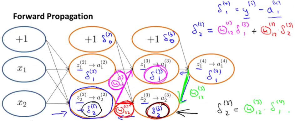
In above, we can compute

$\delta ^{(4)}_1 = y^{(i)} - a^{(4)}_1$

$\delta ^{(3)}_2 = \Theta ^{(3)}_{12} \delta^{(4)}_1$

$\delta ^{(2)}_2 = \Theta ^{(2)}_{12} \delta^{(3)}_1 + \Theta ^{(2)}_{22} \delta^{(3)}_2$

Backpropagation in Practice

Implementation Note: Unrolling Parameters

We use following code to get the optimisation theta.

1
2
3

function [jVal, gradient] = costFunction(theta)
  ...
optTheta = fminunc(@costFunction, initialTheta, options)

Where gradient, theta, initialTheta are vectors of $n+1$ dimension.

In order to use optimizing functions such as fminunc(), we will want to “unroll” all the elements and put them into one long vector:

1
2

thetaVec = [Theta1(:); Theta2(:); Theta3(:)];
DVec = [D1(:); D2(:); D3(:)];

If the dimensions of Theta1 is $10\times11$, Theta2 is $10\times 11$ and Theta3 is $1\times 11$, then we can get back our original matrices from the “unrolled” versions as follows:

1
2
3

Theta1 = reshape(thetaVector(1:110),10,11)
Theta2 = reshape(thetaVector(111:220),10,11)
Theta3 = reshape(thetaVector(221:231),1,11)

Gradient Checking

Gradient checking will assure that our backpropagation works as intended.

Numerical estimation of gradients

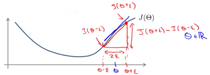
We can approximate the derivative of our cost function with:

$\dfrac{\partial}{\partial\Theta}J(\Theta) \approx \dfrac{J(\Theta + \epsilon) - J(\Theta - \epsilon)}{2\epsilon}$

Implement

1

gradApprox = (J(theta + EPSILON) - J(theta - EPSILON)) / (@ * EPSILON);

Gradient Checking

With multiple theta matrices, we can approximate the derivative with respect to $\Theta _J$ as follows:

$\dfrac{\partial}{\partial\Theta_j}J(\Theta) \approx \dfrac{J(\Theta_1, \dots, \Theta_j + \epsilon, \dots, \Theta_n) - J(\Theta_1, \dots, \Theta_j - \epsilon, \dots, \Theta_n)}{2\epsilon}$

A good small value for ϵ (epsilon), guarantees the math above to become true. If the value be much smaller, may we will end up with numerical problems. The professor Andrew usually uses the value $\epsilon = 10^{-4}$.

Implement

1
2
3
4
5
6
7
8

epsilon = 1e-4;
for i = 1 : n,
  thetaPlus = theta;
  thetaPlus(i) += epsilon;
  thetaMinus = theta;
  thetaMinus(i) -= epsilon;
  gradApprox(i) = (J(thetaPlus) - J(thetaMinus))/(2*epsilon)
end;

We then want to check that gradApprox $\approx$ deltaVector.

Implement Note

• Implement backprop to compute DVec (unrolled $D^{(1)}, D^{(2)}, D^{(3)}$).
• Implement numerical gradient check to compute gradApprox.
• Make sure they give similar values.
• Turn off gradient checking. Using backprop code for learning.

Important

• Be sure to disable your gradient checking code before training your classifier. If you run numerical gradient computation on every iteration of gradient descent (or in the inner loop of costFunction(...)), your code will be very slow.

Random Initialization

Initializing all theta weights to zero does not work with neural networks. When we backpropagate, all nodes will update to the same value repeatedly.

Instead we can randomly initialize our weights to break symmetry.

• Initialize each $\Theta^{(l)}_{ij}$ to a random value between $[-\epsilon, \epsilon]$
  • $\epsilon = \dfrac{\sqrt{6}}{\sqrt{\mathrm{Loutput} + \mathrm{Linput}}}$
  • $\Theta^{(l)} = 2\epsilon\ rand(Loutput, Linput+1)-\epsilon$

1
2
3
4
5

% If the dimensions of Theta1 is 10x11, Theta2 is 10x11 and Theta3 is 1x11.

Theta1 = rand(10,11) * (2 * INIT_EPSILON) - INIT_EPSILON;
Theta2 = rand(10,11) * (2 * INIT_EPSILON) - INIT_EPSILON;
Theta3 = rand(1,11) * (2 * INIT_EPSILON) - INIT_EPSILON;

Note: this epsilon is unrelated to the epsilon from Gradient Checking

Putting It Together

First, pick a network architecture; choose the layout of your neural network, including how many hidden units in each layer and how many layers total.

• Number of input units = dimension of features $x^{(i)}$
• Number of output units = number of classes
• Number of hidden units per layer = usually more the better (must balance with cost of computation as it increases with more hidden units)
• Defaults: 1 hidden layer. If more than 1 hidden layer, then the same number of units in every hidden layer.

Training a Neural Network

1. Randomly initialize the weights
2. Implement forward propagation to get $h_\theta(x^{(i)})$
3. Implement the cost function
4. Implement backpropagation to compute partial derivatives
5. Use gradient checking to confirm that your backpropagation works. Then disable gradient checking.
6. Use gradient descent or a built-in optimization function to minimize the cost function with the weights in theta.

When we perform forward and back propagation, we loop on every training example:

1
2
3

for i = 1:m,
   Perform forward propagation and backpropagation using example (x(i),y(i))
   (Get activations a(l) and delta terms d(l) for l = 2,...,L

Quiz

1. You are training a three layer neural network and would like to use backpropagation to compute the gradient of the cost function. In the backpropagation algorithm, one of the steps is to update $\Delta^{(2)}_{ij} := \Delta^{(2)}_{ij} + \delta^{(3)}_i * (a^{(2)})_j$ for every $i,j$. Which of the following is a correct vectorization of this step?
   • $\Delta(2) :=\Delta(2)+(a(3))^T \ast\delta(2)$
   • $\Delta(2) :=\Delta(2)+\delta(3) \ast (a(3))^T$
   • $\Delta(2) :=\Delta(2)+(a(2))^T \ast \delta(3)$
   • $\Delta(2) :=\Delta(2)+\delta(3) \ast (a(2))^T$
2. Suppose Theta1 is a $5\times 3$ matrix, and Theta2 is a $4\times 6$ matrix. You set thetaVec=[Theta1(:);Theta2(:)]. Which of the following correctly recovers Theta2?
   • reshape(thetaVec(16:39),4,6)
   • reshape(thetaVec(15:38),4,6)
   • reshape(thetaVec(16:24),4,6)
   • reshape(thetaVec(15:39),4,6)
   • reshape(thetaVec(16:39),6,4)
3. Let $J(\theta) = 3\theta^3 + 2$. Let $\theta=1$, and $\epsilon=0.01$. Use the formula $\frac{J(\theta+\epsilon)-J(\theta-\epsilon)}{2\epsilon}$ to numerically compute an approximation to the derivative at $\theta=1$. What value do you get? (When $\theta=1$, the true/exact derivative is $ \frac{d J(\theta)}{ d\theta}=9$.)
   • 9
   • 8.9997
   • 11
   • 9.0003

4. Which of the following statements are true? Check all that apply.

   • Computing the gradient of the cost function in a neural network has the same efficiency when we use backpropagation or when we numerically compute it using the method of gradient checking.
   • For computational efficiency, after we have performed gradient checking to verify that our backpropagation code is correct, we usually disable gradient checking before using backpropagation to train the network.
   • Using gradient checking can help verify if one’s implementation of backpropagation is bug-free.
   • Gradient checking is useful if we are using one of the advanced optimization methods (such as in fminunc) as our optimization algorithm. However, it serves little purpose if we are using gradient descent.
   • Using a large value of $\lambda$ cannot hurt the performance of your neural network; the only reason we do not set $\lambda$ to be too large is to avoid numerical problems.
   • If our neural network overfits the training set, one reasonable step to take is to increase the regularization parameter $\lambda$.
   • Gradient checking is useful if we are using gradient descent as our optimization algorithm. However, it serves little purpose if we are using one of the advanced optimization methods (such as in fminunc).

5. Which of the following statements are true? Check all that apply.

   • Suppose that the parameter $\theta(1)$ is a square matrix (meaning the number of rows equals the number of columns). If we replace $\theta(1)$ with its transpose ($\theta(1)^T$), then we have not changed the function that the network is computing.
   • Suppose we have a correct implementation of backpropagation, and are training a neural network using gradient descent. Suppose we plot $J(\theta)$ as a function of the number of iterations, and find that it is increasing rather than decreasing. One possible cause of this is that the learning rate $\alpha$ is too large.
   • If we are training a neural network using gradient descent, one reasonable “debugging” step to make sure it is working is to plot $J(\theta)$ as a function of the number of iterations, and make sure it is decreasing (or at least non-increasing) after each iteration.
   • Suppose we are using gradient descent with learning rate $\alpha$. For logistic regression and linear regression, $J(\theta)$ was a convex optimization problem and thus we did not want to choose a learning rate $\alpha$ that is too large. For a neural network however, $J(\theta)$ may not be convex, and thus choosing a very large value of $\alpha$ can only speed up convergence.
   • Suppose you have a three layer network with parameters $\theta(1)$ (controlling the function mapping from the inputs to the hidden units) and $\theta(2)$ (controlling the mapping from the hidden units to the outputs). If we set all the elements of $\theta(1)$ to be 0, and all the elements of $\theta(2)$ to be 1, then this suffices for symmetry breaking, since the neurons are no longer all computing the same function of the input.
   • If we initialize all the parameters of a neural network to ones instead of zeros, this will suffice for the purpose of “symmetry breaking” because the parameters are no longer symmetrically equal to zero.