In this post, we are looking into two high-resolution image generation models: ProGAN and StyleGAN. They generates the artificial images gradually, starting from a very low resolution and continuing to a high resolution (finally $1024\times 1024$).

Model Resources
ProGAN [paper] [code (TensorFlow, Official)]
StyleGAN [paper] [code (TensorFlow, Official)]

ProGAN

NVIDIA在2017年底推出的ProGAN解决了GANs生成高质量高分辨率图像的难题。其核心思想在于渐进式的训练方法(Progressive training)。网络从一个非常低的分辨率(如$4\times 4$)开始,逐步训练并增大图像分辨率,直到生成器能够生成的图像分辨率达到目标的高分辨率(如$1024\times 1024$)。

ProGAN从低分辨率到高分辨率的渐进式训练示意图 (Source: Sarah Wolf’s blog post on ProGAN)

使用渐进式生长训练方式的优势在于:

  • 将高分辨率图像生成这样一个复杂的任务,分解为一系列相对简单的任务。这种增量式的学习过程能够很大程度上稳定GANs的训练,并且减少mode collapse现象。
  • 从低分辨率到高分辨率的训练,能够使网络先着眼于在低分辨率图像中也能体现的高层级的图像结构与特征,然后再向其中填充细节。这保证了网络不会在高层级的图像结构中犯大错误,从而提升了生成图像的质量。
  • 此外,渐进生长方式在计算上也比从一开始就训练整个网络的传统方法更为有效。开始时,训练图像分辨率低,网络的层数少,参数量也少,因此网络能够快速收敛。在达到目标分辨率之前,网络都是只有一部分在训练,因此在效率上是有提升的。ProGAN原文中指出,随着目标分辨率的不同,ProGAN的训练速度比传统方法快2至6倍。

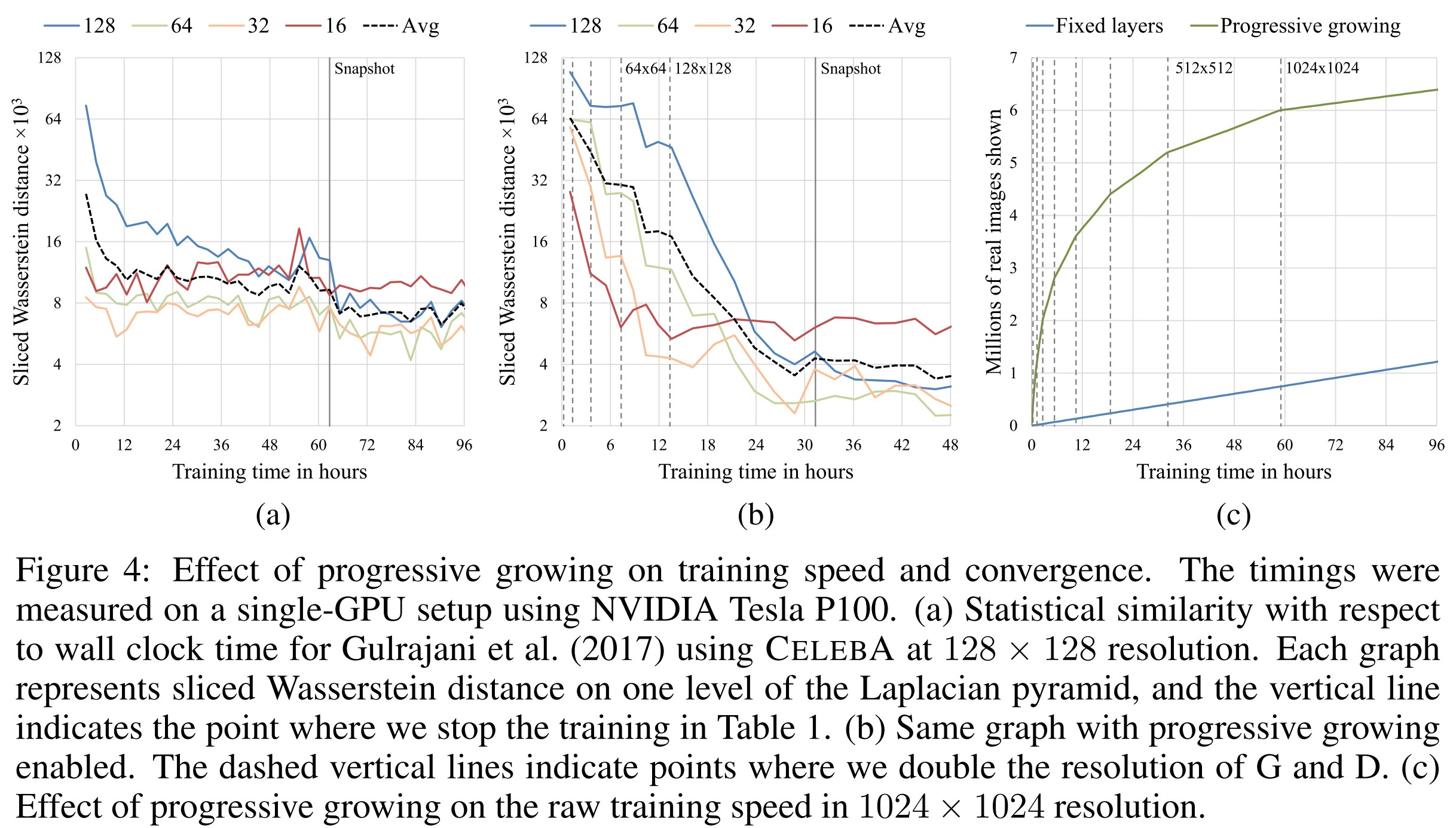
ProGAN训练时间 (Source: original paper)

Workflow

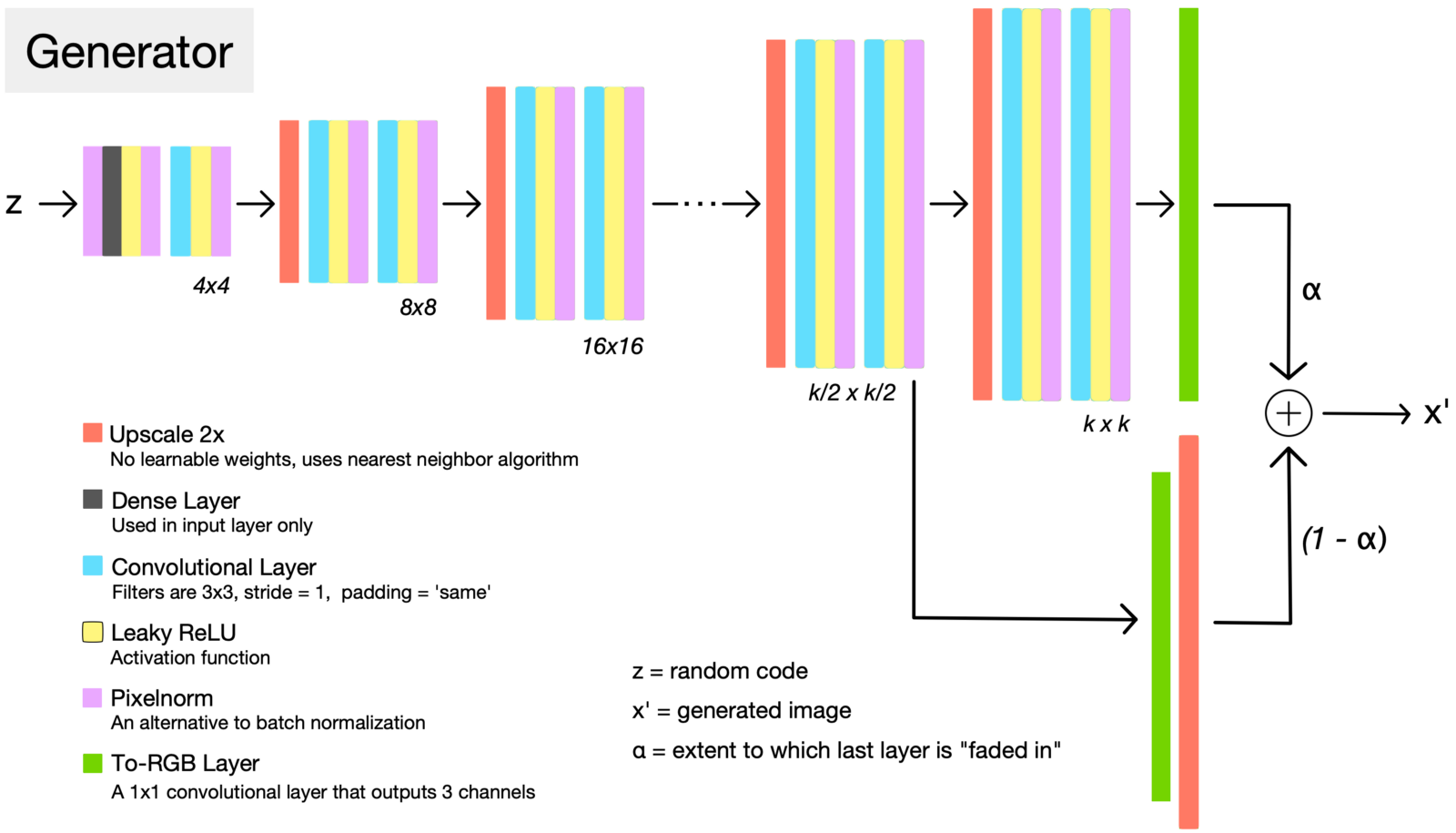
ProGAN网络结构 (Source: original paper)

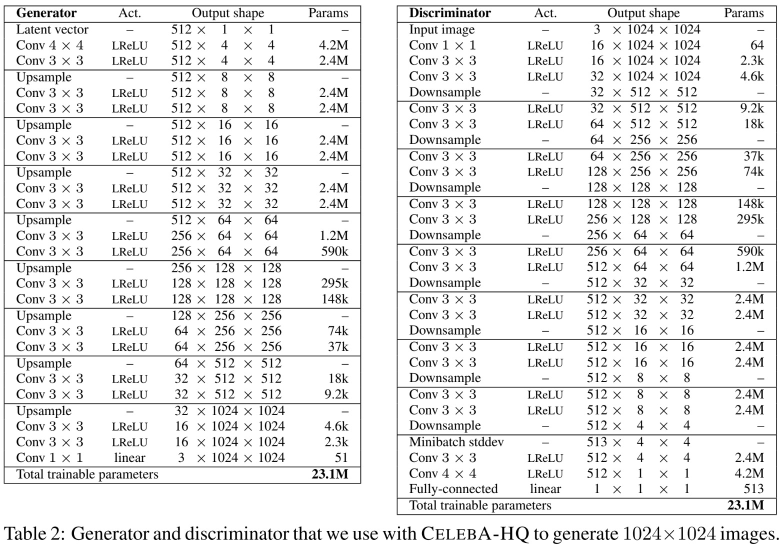
  1. 构建整个ProGAN网络。ProGAN的网络架构是多尺度的。Generator的每一组都将空间尺寸扩大到原先的两倍,通道数则减少为原先的一半。直到特征的空间尺寸达到目标尺寸,通道数则减少到$3$,及RGB三个通道。Discriminator的网络结构则基本上是Generator的镜像,每一组都减半空间尺寸,倍增通道数。同时,为了保证总参数量不至于过高,倍增得到的通道数的上限设为$512$。
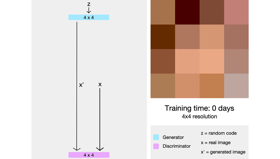
  2. 按照分辨率从低到高逐步训练ProGAN网络。从$4\times 4​$的网络开始训练,稳定后增长分辨率,Generator与Discriminator同时增加一组卷积层,首先进入Fade-in模式,之后进入Stabilize模式。当增加新的卷积层后,原有层内的参数仍然保持可训练的状态。稳定后,继续增大分辨率,如上述进行训练。如此反复,直到达到目标分辨率。

Details

Fading in new layers

ProGAN网络Generator结构与增长分辨率时的Fade-in策略 (Source: Sarah Wolf’s blog post on ProGAN)

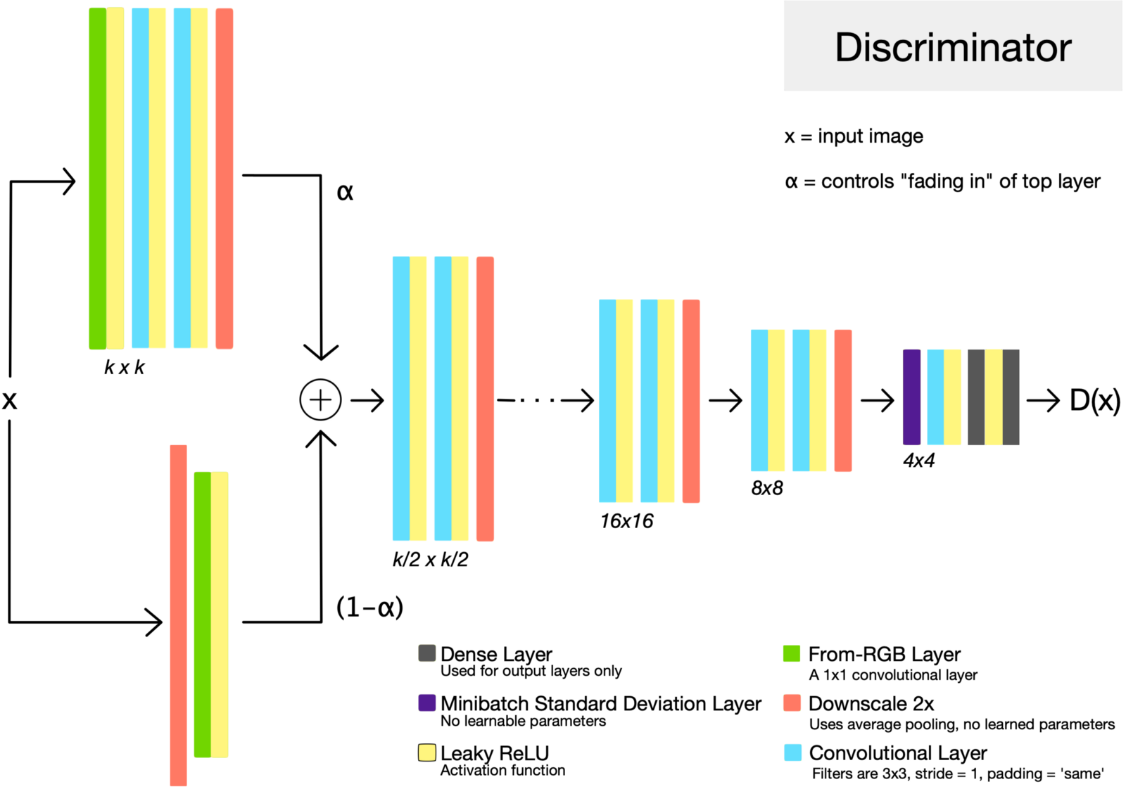
ProGAN网络Discriminator结构 (Source: Sarah Wolf’s blog post on ProGAN

当增大分辨率时,Generator与Discriminator都会增加卷积层。为了让新加层快速收敛,同时又不对原有层造成过大的影响,ProGAN提出了一种Fade-in的机制。如上图所示,在Fade-in阶段时,旧有的层的输出经过上采样放大两倍,而后通过toRGB层转化为RGB图像,与新加层的输出通过toRGB层转化后的图像进行加权和,形成最终的输出。这一融合由一个参数$\alpha​$进行控制,$x'=\alpha x_{i} + (1-\alpha) x_{i-1}$。随着训练的进行,$\alpha​$从$1​$线性减少为$0​$,最终输出也逐渐转为新加层的输出占主导。

 1
 2
 3
 4
 5
 6
 7
 8
 9
10
11
12
13
# fade-in phase in generator
upsample = F.interpolate(out, scale_factor=2, mode='nearest', align_corners=False)
out = self.progression[i](out)
out = self.to_rgb[i](out)
skip_rgb = self.to_rgb[i - 1](upsample)
out = (1 - alpha) * skip_rgb + alpha * out

# fade-in phase in discriminator
out = self.progression[i](out)
out = F.avg_pool2d(out, 2)
downsample = F.avg_pool2d(input, 2)
skip_rgb = self.from_rgb[i + 1](downsample)
out = (1 - alpha) * skip_rgb + alpha * out

Minibatch Standard Deviation

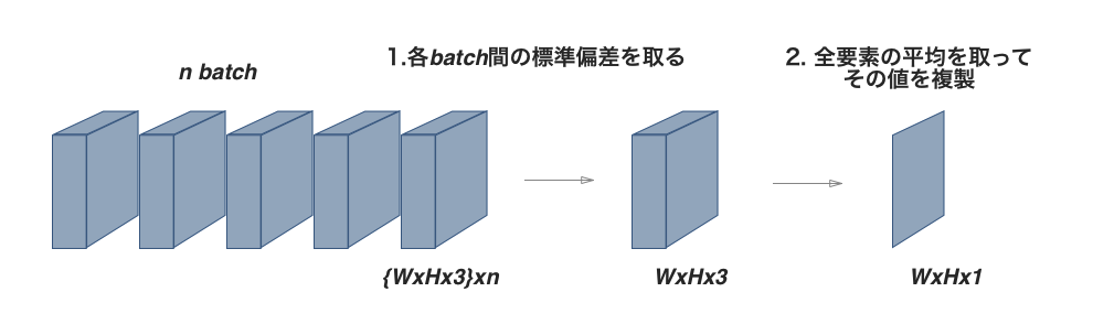
ProGAN网络Discrimiantor中的minibatch standard deviation层 (Source: [DL輪読会]Progressive Growing of GANs for Improved Quality, Stability, and Variation))

ProGAN为了解决GANs生成的图像多样性较差的问题,在discriminator的最后增加了一个minibatch standard deviation层。 这个层没有需要训练的参数,其作用为求取minibatch内的所有feature maps ($N\times C\times H\times W$)上各个像素位置对应的标准差($C\times H\times W$),再求其平均值($\text{scalar}$),将其展开为一张新的feature map ($N \times 1\times H\times W$)作为新的通道加入。这有助于统计minibatch内的信息,让discriminator根据这些额外的统计信息来区分真是样本的batch与生成样本的batch。从而让generator需要生成更加多样化、更加接近真实样本分布的样本来“骗过”discriminator,最终达到增强generator生成多样化样本的目的。

1
2
3
4
out_std = torch.sqrt(out.var(0, unbiased=False) + 1e-8)
mean_std = out_std.mean()
mean_std = mean_std.expand(out.size(0), 1, 4, 4)
out = torch.cat([out, mean_std], 1)

toRGB & fromRGB

在训练过程中,Generator的输出以及Discriminator的输入需要为RGB图像,这就需要使用$1\times 1$的卷积将在多通道的feature maps与3通道的图像之间进行转换。这就是toRGB(Generator最后一层卷积层)与fromRGB层(Discriminator第一层卷积层)的由来。当然,针对不同分辨率的toRGB层与fromRGB层是不同尺寸的,且是单独训练的。

 1
 2
 3
 4
 5
 6
 7
 8
 9
10
11
12
13
14
# toRGB layers in generator
to_rgb = nn.ModuleList([EqualConv2d(512, 3, 1),
                        EqualConv2d(512, 3, 1),
                        EqualConv2d(512, 3, 1),
                        EqualConv2d(512, 3, 1),
                        EqualConv2d(256, 3, 1),
                        EqualConv2d(128, 3, 1)])
# fromRGB layers in discriminator
from_rgb = nn.ModuleList([EqualConv2d(3, 128, 1),
                          EqualConv2d(3, 256, 1),
                          EqualConv2d(3, 512, 1),
                          EqualConv2d(3, 512, 1),
                          EqualConv2d(3, 512, 1),
                          EqualConv2d(3, 512, 1)])

Loss function

ProGAN使用的是WGAN-GP,介绍可参见之前的文章。其损失函数形式为:

$$ \begin{aligned} \mathcal{L}_G &= -D(x') \\ \mathcal{L}_D &= -D(x) + D(x') + \lambda \times GP \\ GP &= \left(||\nabla D (\alpha x' + (1 - \alpha)x ))||_2 - 1 \right)^2 \\ \end{aligned} $$

其中,$D$为Discriminator,$x$、$x’$分别为真实样本与生成样本。$\lambda=10$为权重项,$GP$为用于稳定训练的梯度惩罚项,$\alpha \in (0,1)$为均匀采样的随机数,用以表示$x$与$x’$的加权平均(即其连线上的任意一点)。

Tricks

Upscale 2x

在放大特征图的方法上,与DCGAN等使用转置卷积(transpose convolutions)不同,ProGAN用最近邻插值来视线上采样,用average pooling来降采样。这两种方法均不需要可学习的参数,更为简单。

1
2
3
4
5
6
7
from torch import nn
from torch.nn import functional as F

# upsample = nn.F.interpolate(out, scale_factor=2, mode='nearest', align_corners=False)
upsampler = nn.UpsamplingNearest2d(scale_factor=2)
# downsample = F.avg_pool2d(out, 2)
downsampler = torch.nn.AvgPool2d(kernel_size=2)

Equalized Learning Rate

为了保证Generator与Discriminator之间的良性竞争,ProGAN指出需要使得各个卷积层以相似的速度进行学习。为了达到equlized learnig rate,ProGAN采用了与He initialization相似的方法,也就是将每个层的权重乘以其权重参数量。而且不仅仅是初始化权重时这么做,在训练过程的每次forwarding时都进行此操作。

$$ W = W_{orig} \times \sqrt{\frac{2}{\text{fan_in}}} $$

其中$W_{orig}$、$W$分别为原始权重与实际使用的权重,对于卷积层来说,$\text{fan_in} = k\times k \times c$,$k$为kernel大小,$c$为通道数。

 1
 2
 3
 4
 5
 6
 7
 8
 9
10
11
12
13
14
15
16
17
18
19
20
21
22
23
24
25
26
27
28
29
30
31
32
33
34
35
36
37
38
39
40
41
class EqualLR:
    def __init__(self, name):
        self.name = name

    def compute_weight(self, module):
        weight = getattr(module, self.name + '_orig')
        fan_in = weight.data.size(1) * weight.data[0][0].numel()

        return weight * sqrt(2 / fan_in)

    @staticmethod
    def apply(module, name):
        fn = EqualLR(name)

        weight = getattr(module, name)
        del module._parameters[name]
        module.register_parameter(name + '_orig', nn.Parameter(weight.data))
        module.register_forward_pre_hook(fn)
        return fn

    def __call__(self, module, input_tensor):
        weight = self.compute_weight(module)
        setattr(module, self.name, weight)


def equal_lr(module, name='weight'):
    EqualLR.apply(module, name)
    return module


class EqualConv2d(nn.Module):
    def __init__(self, *args, **kwargs):
        super().__init__()

        conv = nn.Conv2d(*args, **kwargs)
        conv.weight.data.normal_()
        conv.bias.data.zero_()
        self.conv = equal_lr(conv)

    def forward(self, input_tensor):
        return self.conv(input_tensor)

Pixel Normalization

ProGAN没有使用BN层,而是提出了Pixel Normalization层。与BN层类似,PN层直接放在卷积层之后,激活函数之前。这个层没有需要训练的参数,其作用为将feature maps中的每个像素位置$(x,y)$在不同的通道$C​$上的值都归一化到单位长度:

$$ b_{x,y} = \frac{a_{x,y}}{\sqrt{\frac{1}{C} \sum^C_{j=0} a_{x,y}^j+\epsilon}} $$

其中,$a$、$b$分别为输入张量与输出张量,$\epsilon=10^{-8}$为防止除以零的常数。这一举措能够防止像素位置上的信号响应在训练过程中失控,可以提升训练时的稳定性。

1
2
3
4
5
6
7
class PixelNorm(nn.Module):
    def __init__(self):
        super().__init__()

    def forward(self, input_tensor):
        return input_tensor / torch.sqrt(
            torch.mean(input_tensor ** 2, dim=1, keepdim=True) + 1e-8)

Drawbacks

ProGAN虽然能够生成高质量高分辨率的图像,但是其本质上还是一种无条件(unconditional)的生成方法。其难以控制所生成图像的属性。并且就算是修改输入的随机向量,其微小的变化也会引起最终生成图像中的多个属性一起变化。如何将ProGAN改为有条件(conditional)的生成模型,或者增强其微调单个属性的能力,这是一个可以研究的方向。

StyleGAN

StyleGAN是NVIDIA继ProGAN之后提出的新的生成网络,其主要通过分别修改每一层级的输入,在不影响其他层级的情况下,来控制该层级所表示的视觉特征。这些特征可以是粗的特征(如姿势、脸型等),也可以是一些细节特征(如瞳色、发色等)。

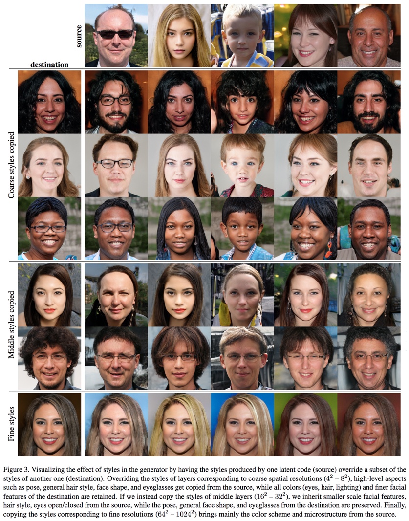
StyleGAN可视化结果 (Source: original paper)

具体地说,StyleGAN提出,如果训练得当,ProGAN的每一个层级都有能力控制不同的视觉特征。层级越低,分辨率越低,其能控制的视觉特征也就越粗糙。因此,StyleGAN将视觉特征划分为三类:

  1. 粗糙(初级)特征:分辨率小于$8\times 8$,主要影响姿态、大致发型、脸型等;
  2. 中级特征:分辨率介于$16\times 16$至$32\times 32$之间,主要影响更加细节的脸部特征、细节发型、嘴的张闭等;
  3. 细节(高级)特征:分辨率介于$64\times 64$至$1024\times 1024​$之间,主要影响整体的色调(发色、肤色以及背景色等)与一些细微的特征。

Workflow

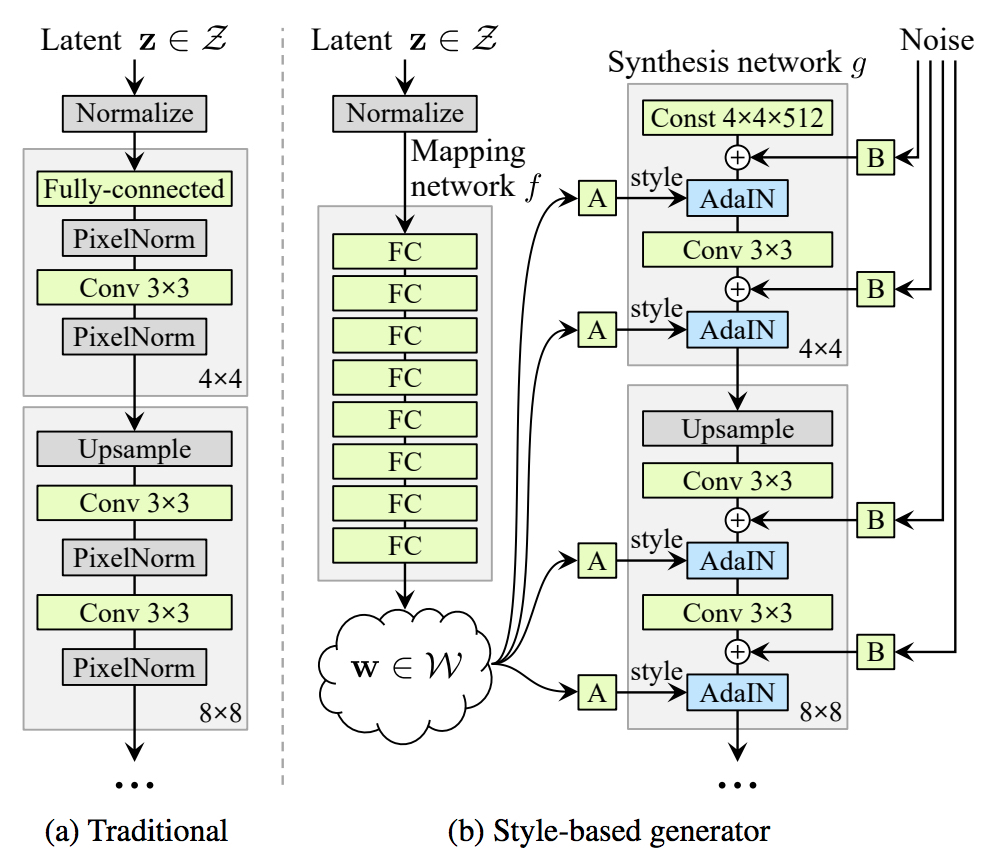
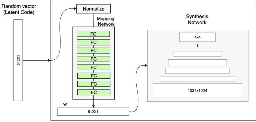
StyleGAN网络结构 (Source: original paper)

  1. 从先验分布$\mathcal{Z}$中采样一个一个$512\times 1$的随机向量$\mathbf{z} \in \mathcal{Z}$作为latent code,归一化后经过Mapping Network映射到另外一个中间的latent space上,得到中间的latent code表示$\mathbf{w} \in \mathcal{W}$
  2. 将上一步得到的$\mathbf{w}$通过可学习的仿射变换$A$输入到Synthesis Network各个层级的AdaIN层中中,用以控制style;同时将噪声通过学习到的缩放参数$B$加到AdaIN层之前
  3. 将固定的向量输入Synthesis Network,输出得到生成的图像。
 1
 2
 3
 4
 5
 6
 7
 8
 9
10
11
12
13
14
15
16
17
18
19
20
21
22
23
24
25
26
27
28
29
30
31
32
33
34
35
36
37
38
39
40
41
42
43
44
45
46
47
48
49
50
51
52
53
54
55
56
class StyledConvBlock(nn.Module):
    def __init__(self, in_channel, out_channel, kernel_size=3,
                 padding=1, style_dim=512, initial=False):
        super().__init__()

        if initial:
            self.conv1 = ConstantInput(in_channel)

        else:
            self.conv1 = EqualConv2d(in_channel, out_channel, kernel_size, padding=padding)

        self.noise1 = equal_lr(NoiseInjection(out_channel))
        self.adain1 = AdaptiveInstanceNorm(out_channel, style_dim)
        self.lrelu1 = nn.LeakyReLU(0.2)

        self.conv2 = EqualConv2d(out_channel, out_channel, kernel_size, padding=padding)
        self.noise2 = equal_lr(NoiseInjection(out_channel))
        self.adain2 = AdaptiveInstanceNorm(out_channel, style_dim)
        self.lrelu2 = nn.LeakyReLU(0.2)

    def forward(self, input, style, noise):
        out = self.conv1(input)
        out = self.noise1(out, noise)
        out = self.adain1(out, style)
        out = self.lrelu1(out)

        out = self.conv2(out)
        out = self.noise2(out, noise)
        out = self.adain2(out, style)
        out = self.lrelu2(out)

        return out
    
    
class Generator(nn.Module):
    def __init__(self, code_dim):
        super().__init__()

        self.progression = nn.ModuleList([StyledConvBlock(512, 512, 3, 1, initial=True),
                                          StyledConvBlock(512, 512, 3, 1),
                                          StyledConvBlock(512, 512, 3, 1),
                                          StyledConvBlock(512, 512, 3, 1),
                                          StyledConvBlock(512, 256, 3, 1),
                                          StyledConvBlock(256, 128, 3, 1)])

        self.to_rgb = nn.ModuleList([EqualConv2d(512, 3, 1),
                                     EqualConv2d(512, 3, 1),
                                     EqualConv2d(512, 3, 1),
                                     EqualConv2d(512, 3, 1),
                                     EqualConv2d(256, 3, 1),
                                     EqualConv2d(128, 3, 1)])

        # self.blur = Blur()

    def forward(self, style, noise, step=0, alpha=-1, mixing_range=(-1, -1)):
        pass

Details

Mapping Network

Mapping Network的作用是将输入向量编码为一个中间表示,使得该中间表示的每一个元素都能够控制不同的视觉特征。

如果像传统的cGANs及其衍生版本那样,只靠输入向量自身控制视觉特征,这种能力是有限的,因为其还要受到训练数据的概率密度分布的影响。训练数据中如果某一类出现得多一些,那么输入向量中的值就更可能被映射到这一类上面。这就导致了模型所控制的特征是耦合的(coupled)或者说是纠缠的(entangled),模型并不能单独控制输入向量的某一部分的映射。但是通过Mapping Network将输入向量映射为另外的中间表示,则不用服从训练数据集的分布,并且能够在一定程度上减少特征之间的相关性。

Mapping Network由8层FC层组成,输入为随机向量$\mathbf{z} \in \mathcal{Z}$,输出为中间表示$\mathbf{w} \in \mathcal{W}$,两者维度均为$512\times 1$。

StyleGAN网络中的Mapping Network (Source: Rani Horev's blog post)

 1
 2
 3
 4
 5
 6
 7
 8
 9
10
11
12
13
14
15
class StyledGenerator(nn.Module):
    def __init__(self, code_dim=512, n_mlp=8):
        super().__init__()

        self.generator = Generator(code_dim)

        layers = [PixelNorm()]
        for i in range(n_mlp):
            layers.append(EqualLinear(code_dim, code_dim))
            layers.append(nn.LeakyReLU(0.2))

        self.style = nn.Sequential(*layers)

    def forward(self, input, noise=None, step=0, alpha=-1, mean_style=None, style_weight=0, mixing_range=(-1, -1)):
		pass

Adaptive Instance Normalization (AdaIN)

Mapping Network编码得到的中间表示$\mathbf{w} \in \mathcal{W}$,需要通过AdaIN (Adaptive Instance Normalization)来输入生成网络。AdaIN层在Systhesis Network的每个分辨率层级中都存在,并且用以控制该分辨率层级的视觉特征。

$$ \text{AdaIN}(x_i,y) = y_{s,i} \frac{x_i - \mu(x_i)}{\sigma(x_i)} + y_{b,i} $$
  1. 对卷积层的输出进行Instance Normalization,也就是将输出的每个通道都进行归一化,得到$\frac{x_i - \mu(x_i)}{\sigma(x_i)}$
  2. 对输入的中间表示$\mathbf{w}$(维度$512$)通过一个FC层$A$转换为针对$n$个通道的scale ($y_{s,i}$)与bias ($y_{b,i}$),维度为$2n$
  3. 通过第2步得到的scale与bias,对于第1步得到的归一化输出的每个通道都进行shift。这种操作相当于对卷积层的每个滤波器的输出进行加权,而这个权重是可学习的。通过训练,使得$\mathbf{w}$所代表的权重能够被转化为视觉表示。

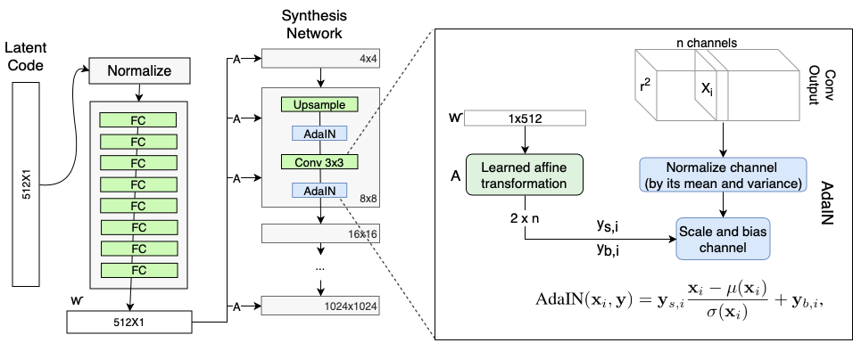
StyleGAN网络中的AdaIN模块 (Source: Rani Horev's blog post)

 1
 2
 3
 4
 5
 6
 7
 8
 9
10
11
12
13
14
15
16
17
18
19
20
class AdaptiveInstanceNorm(nn.Module):
    def __init__(self, in_channel, style_dim):
        super().__init__()

        self.norm = nn.InstanceNorm2d(in_channel)
        self.style = EqualLinear(style_dim, in_channel * 2)

        self.style.linear.bias.data[:in_channel] = 1
        self.style.linear.bias.data[in_channel:] = 0

    def forward(self, input, style):
        # 512 -> Nx2
        style = self.style(style).unsqueeze(2).unsqueeze(3)
        # split sytle inyo scale and bias
        gamma, beta = style.chunk(2, 1)

        out = self.norm(input)
        out = gamma * out + beta

        return out

Removing traditional input

包含之前的ProGAN在内,传统的GANs都需要用一个随机向量喂给生成网络来生成图像,这个随机向量就决定了生成图像的视觉特征。而在StyleGAN中,既然生成图像的视觉特征已经交由$\mathbf{w}$与AdaIn来控制,那么再在Synthesis Network的最开始输入一个随机向量就显得有点多余了。因此这个随机向量输入被替换成了一个定值向量输入,而且这在结果上有益于生成图像的质量。一个可能的解释是这种固定的输入使得网络只需要考虑$\mathbf{w}$那边传过来的视觉属性,而不用再管另外一个输入的变量,从而在一定程度上减少特征之间的纠缠。

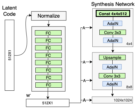
StyleGAN网络在Synthesis Network上使用了固定的输入 (Source: Rani Horev's blog post)

 1
 2
 3
 4
 5
 6
 7
 8
 9
10
11
12
13
class ConstantInput(nn.Module):
    def __init__(self, channel, size=4):
        super().__init__()
		
        # generate fixed random vector
        self.input = nn.Parameter(torch.randn(1, channel, size, size))

    def forward(self, input):
        # generate fake batch
        batch = input.shape[0]
        out = self.input.repeat(batch, 1, 1, 1)

        return out

Stochastic variation

为了增强生成样本的多样性,同时考虑到人脸上还是有许多地方可以看成是随机的(例如雀斑、皱纹、头发纹理等等),通常GANs会在输入向量上增加一层随机噪声来实现这种微小的特征。StyleGAN也一样,如果只使用$\mathbf{w}$来控制视觉特征,输入Synthesis Network的向量又是固定的,那么一旦$\mathbf{w}$固定,则生成的图像也是一成不变的。

不过,如上文所述,传统方法直接将随机噪声加在输入变量上,这样容易导致特征的纠缠现象,使得其他的特征也受到影响。同样地,与上面的解决方法一致,StyleGAN将噪声通过FC层$B$重新编码,然后加在AdaIN之前一层输出的每个通道上,用以轻微改变每一层级所负责的视觉特征。

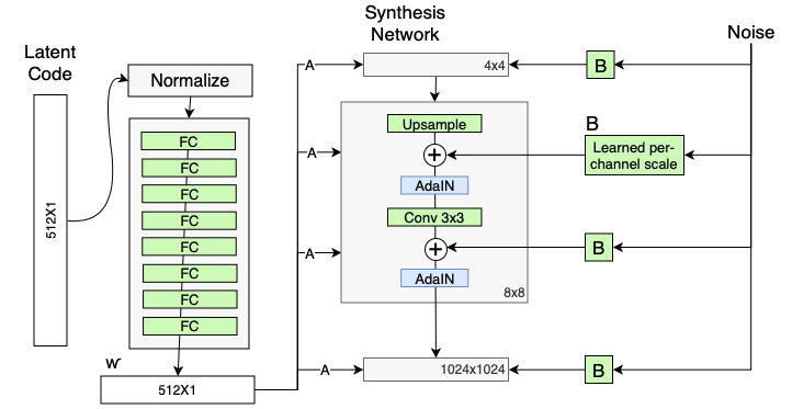
StyleGAN网络在AdaIN层之前增加了编码后的噪声 (Source: Rani Horev's blog post)

1
2
3
4
5
6
7
8
class NoiseInjection(nn.Module):
    def __init__(self, channel):
        super().__init__()

        self.weight = nn.Parameter(torch.zeros(1, channel, 1, 1))

    def forward(self, image, noise):
        return image + self.weight * noise

Tricks

Style Mixing

(to be continued)

Reference